Exponential integrals, and related functions

Exponential integral \(E_1(x)\)

ctx.exp_integral_e1(x)

where ctx is math53 or ctxflint.

Returns the exponential integral \(\displaystyle E_1(x) = \int_1^\infty \frac{e^{-xt}}{t} \, \mathrm{d}t, = e^{-z} U(1,1,z), \quad x \neq 0\).

For real \(x<0\) the integral can be calculated as \(E_1(x) = -\mathrm{Ei}(-x)\).

See also Wikipedia [1427], MathWorld [1052], NIST [844], BoostMath [160], Ehrhardt [309] (3.4.5), Ehrhardt [309] (4.2.27), Flint [839], Flint [832], Mpmath [682].

An example in Python

>>> from xlcalcnet import ereal
>>> ereal.E1(0.5)
ereal('5.2359877559829887307E-1')
>>> ereal.E1('0.51')
ereal('5.3518479027559984754E-1')

An example with real input:

>>> from xlcalcnet import dec, mpm, gmp, fpm, apm
>>> mpm.dps = 40; x = 3.0
>>> \mathrm{d}x = dec.e1(x); mx = mpm.e1(x); gx = gmp.e1(x)
>>> fx = fpm.e1(x); ax = apm.e1(x)
>>> mpm.show([\mathrm{d}x, mx, gx, fx, ax])
dec:  1.304838109419703741250074582864502294848E-2
mpm:  1.304838109419703741250074582864502294848e-2
gmp:  1.304838109419703741250074582864502294848E-02
fpm:  1.30483810941970E-02
apm:  1.304838109419703741250074582864502294848e-2 (8.248e-39%)

An example with complex input:

>>> from xlcalcnet import dec, mpm, gmp, fpm, apm
>>> mpm.dps = 20; z = '3.0 + 4.0j'
>>> \mathrm{d}z = dec.e1(z); mz = mpm.e1(z); gz = gmp.e1(z)
>>> fz = fpm.e1(z); az = apm.e1(z)
>>> mpm.show([\mathrm{d}z, mz, gz, fz, az], aligned=True)
dec: 8.6395395897958511158E-4              + 8.7862083771974420418E-3j
mpm: 8.6395395897958511158e-4              + 8.7862083771974420418e-3j
gmp: 8.6395395897958511158E-04             + 8.7862083771974420418E-03j
fpm: 8.63953958979585E-04                  + 8.78620837719744E-03j
apm: 8.6395395897958511148e-4 (8.234e-17%) + 8.7862083771974420418e-3 (7.381e-18%)j

Exponential integral \(\mathrm{Ei}(x)\)

ctx.exp_integral_ei(x)

where ctx is math53, mathc53, ctxboost or ctxflint.

Returns the exponential integral \(\displaystyle \mathrm{Ei}(x) = -PV \int_{-x}^\infty \frac{e^{-t}}{t} \, \mathrm{d}t= PV \int_{-\infty}^x \frac{e^{t}}{t} \, \mathrm{d}t\).

For real \(x<0\) we have \(\mathrm{Ei}(x) = -E_1(-x)\).

See also Wikipedia [1427], MathWorld [1052], NIST [844], BoostMath [160], Ehrhardt [309] (3.4.7), Ehrhardt [309] (4.2.27), Flint [839], Flint [832], Mpmath [683].

The exponential integral \(\mathrm{Ei}(z)\) can also be calculated as using

\[\mathrm{Ei}(z) = -e^z U(1,1,-z) - \log(-z) + \frac{1}{2} \left(\log(z) - \log\left(\frac{1}{z}\right) \right)\]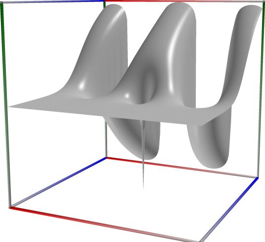

\(\quad\) \(\quad\)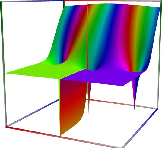

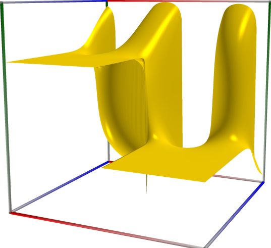
3D wpf plot: real part (left figure), imaginary part (middle figure) and absolute value with color-coded phase (right figure) of the complex sine function \(z = \sin(x + iy)\), with \(-6 \le x \le 6\) (blue axis), \(-6 \le y \le 6\) (red axis), \(-10 \le z \le 10\) (green axis). Function values are loglog-transformed.

An example in Python

>>> from xlcalcnet import ereal
>>> ereal.Ei(0.5)
ereal('5.2359877559829887307E-1')
>>> ereal.Ei('0.51')
ereal('5.3518479027559984754E-1')

An example with real input:

>>> from xlcalcnet import dec, mpm, gmp, fpm, apm
>>> mpm.dps = 40; x = 3.0
>>> \mathrm{d}x = dec.ei(x); mx = mpm.ei(x); gx = gmp.ei(x)
>>> fx = fpm.ei(x); ax = apm.ei(x)
>>> mpm.show([\mathrm{d}x, mx, gx, fx, ax])
dec:  9.933832570625416558008336019216765262991E+0
mpm:  9.933832570625416558008336019216765262991e+0
gmp:  9.933832570625416558008336019216765262991E+00
fpm:  9.93383257062542E+00
apm:  9.933832570625416558008336019216765262991e+0 (9.245e-40%)

An example with complex input:

>>> from xlcalcnet import dec, mpm, gmp, fpm, apm
>>> mpm.dps = 20; z = '3.0 + 4.0j'
>>> \mathrm{d}z = dec.ei(z); mz = mpm.ei(z); gz = gmp.ei(z)
>>> fz = fpm.ei(z); az = apm.ei(z)
>>> mpm.show([\mathrm{d}z, mz, gz, fz, az], aligned=True)
dec: -4.1540916516426898225E+0               + 4.2944186200243574770E+0j
mpm: -4.1540916516426898225e+0               + 4.2944186200243574770e+0j
gmp: -4.1540916516426898225E+00              + 4.2944186200243574770E+00j
fpm: -4.15409165164269E+00                   + 4.29441862002436E+00j
apm: -4.1540916516426898225e+0 (-8.156e-20%) + 4.2944186200243574770e+0 (7.89e-20%)j

Logarithmic integral \(\mathrm{li}(x)\)

ctx.log_integral(z)

where ctx is math53, mathc53 or ctxflint.

Returns the logarithmic integral \(\displaystyle \mathrm{li}(x) = PV \int_{0}^{x} \frac{1}{\log(t)} \, \mathrm{d}t, \quad (x \geq 0, x \neq 1)\).

For \(x \neq 0\) the integral is calculated as \(\mathrm{li}(x)=\mathrm{Ei}(\log(x))\).

See also Wikipedia [1436], MathWorld [1063], NIST [847], Ehrhardt [309] (3.4.15), Ehrhardt [309] (4.2.40), Flint [839], Flint [832], Mpmath [691].

\(\quad\) \(\quad\)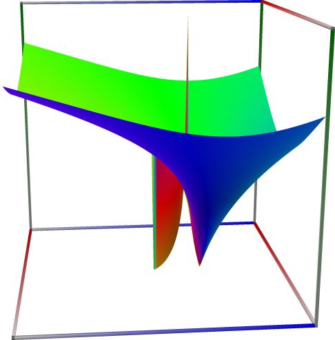

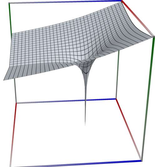
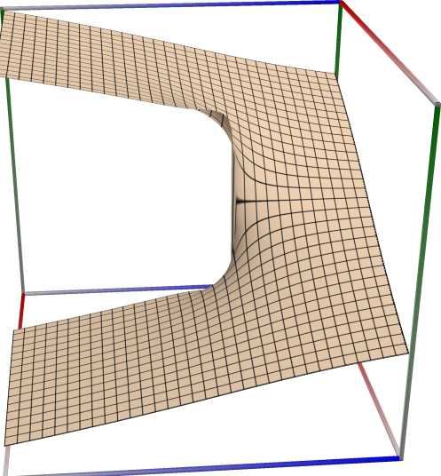
3D wpf plot: real part (left figure), imaginary part (middle figure) and absolute value with color-coded phase (right figure) of the complex sine function \(z = \sin(x + iy)\), with \(-6 \le x \le 6\) (blue axis), \(-6 \le y \le 6\) (red axis), \(-10 \le z \le 10\) (green axis). Function values are loglog-transformed.

An example in Python

>>> from xlcalcnet import ereal
>>> ereal.Li(0.5)
ereal('5.2359877559829887307E-1')
>>> ereal.Li('0.51')
ereal('5.3518479027559984754E-1')

An example with real input:

>>> from xlcalcnet import dec, mpm, gmp, fpm, apm
>>> mpm.dps = 40; x = 3.0
>>> \mathrm{d}x = dec.li(x); mx = mpm.li(x); gx = gmp.li(x)
>>> fx = fpm.li(x); ax = apm.li(x)
>>> mpm.show([\mathrm{d}x, mx, gx, fx, ax])
dec:  2.163588594667191972876922367347721366542E+0
mpm:  2.163588594667191972876922367347721366542e+0
gmp:  2.163588594667191972876922367347721366542E+00
fpm:  2.16358859466719E+00
apm:  2.163588594667191972876922367347721366542e+0 (1.061e-39%)

An example with complex input:

>>> from xlcalcnet import dec, mpm, gmp, fpm, apm
>>> mpm.dps = 20; z = '3.0 + 4.0j'
>>> \mathrm{d}z = dec.li(z); mz = mpm.li(z); gz = gmp.li(z)
>>> fz = fpm.li(z); az = apm.li(z)
>>> mpm.show([\mathrm{d}z, mz, gz, fz, az], aligned=True)
dec: 3.1343755504645775265E+0              + 2.6769247817778742392E+0j
mpm: 3.1343755504645775265e+0              + 2.6769247817778742392e+0j
gmp: 3.1343755504645775265E+00             + 2.6769247817778742392E+00j
fpm: 3.13437555046458E+00                  + 2.67692478177787E+00j
apm: 3.1343755504645775265e+0 (1.081e-19%) + 2.6769247817778742392e+0 (6.328e-20%)j

Hyperbolic sine integral \(\mathrm{Shi}(x)\)

ctx.sinh_integral(x)

where ctx is math53, ctxflint.

Returns the hyperbolic sine integral \(\displaystyle \mathrm{Shi}(x) = \int_0^x \frac{\sinh(t)}{t} \, \mathrm{d}t\).

See also Wikipedia [1433], MathWorld [1059], NIST [846], Ehrhardt [309] (3.4.17), Flint [839], Flint [832], Mpmath [694].

For real \(x\) the integral is calculated using the relations \(\displaystyle \text{Shi}(x) = \tfrac{1}{2} \left(\text{Ei}(x)+\text{E}_1(x)\right)\) for \(x>0\) and \(\mathrm{Shi}(x) = -\mathrm{Shi}(-x)\) for \(x<0\).

For complex \(x\) the integral is calculated using the relation \(\displaystyle \text{Shi}(x) = -i \text{Si}(ix)\).

An example in Python

>>> from xlcalcnet import ereal
>>> ereal.Shi(0.5)
ereal('5.2359877559829887307E-1')
>>> ereal.Shi('0.51')
ereal('5.3518479027559984754E-1')

An example with real input:

>>> from xlcalcnet import dec, mpm, gmp, fpm, apm
>>> mpm.dps = 40; x = 3.0
>>> \mathrm{d}x = dec.shi(x); mx = mpm.shi(x); gx = gmp.shi(x)
>>> fx = fpm.shi(x); ax = apm.shi(x)
>>> mpm.show([\mathrm{d}x, mx, gx, fx, ax])
dec:  4.973440475859806797710418382522705142970E+0
mpm:  4.973440475859806797710418382522705142970e+0
gmp:  4.973440475859806797710418382522705142970E+00
fpm:  4.97344047585981E+00
apm:  4.973440475859806797710418382522705142970e+0 (9.233e-40%)

An example with complex input:

>>> from xlcalcnet import dec, mpm, gmp, fpm, apm
>>> mpm.dps = 20; z = '3.0 + 4.0j'
>>> \mathrm{d}z = dec.shi(z); mz = mpm.shi(z); gz = gmp.shi(z)
>>> fz = fpm.shi(z); az = apm.shi(z)
>>> mpm.show([\mathrm{d}z, mz, gz, fz, az], aligned=True)
dec: -2.0766138488418551187E+0               + 2.1516024142007774595E+0j
mpm: -2.0766138488418551187e+0               + 2.1516024142007774595e+0j
gmp: -2.0766138488418551187E+00              + 2.1516024142007774595E+00j
fpm: -2.07661384884186E+00                   + 2.15160241420078E+00j
apm: -2.0766138488418551187e+0 (-1.632e-19%) + 2.1516024142007774595e+0 (7.874e-20%)j

Hyperbolic cosine integral \(\mathrm{Chi}(x)\)

ctx.cosh_integral(x)

where ctx is math53, ctxflint.

Note: Also math53.chi(z), ctx.coshIntegral(z)

Returns the hyperbolic cosine integral \(\displaystyle \mathrm{Chi}(x) = -\int_x^{\infty} \frac{\cosh(t)}{t} \, \mathrm{d}t = \gamma + \log(x) + \int_0^x \frac{\cosh(t) - 1}{t} \, \mathrm{d}t\).

See also Wikipedia [1432], MathWorld [1058], NIST [846], Ehrhardt [309] (3.4.1), Flint [839], Flint [832], Mpmath [678].

For real \(x\) the integral is calculated using the relations \(\displaystyle \text{Chi}(x) = \tfrac{1}{2} \left(\text{Ei}(x)-\text{E}_1(x)\right)\) for \(x>0\) and \(\text{Chi}(x) = \text{Chi}(-x)\) for \(x<0\).

For complex \(x\) the integral is calculated using the relation \(\displaystyle \text{Chi}(x) = \text{Ci}(i x) - \log(i x) + \log(x)\).

An example in Python

>>> from xlcalcnet import ereal
>>> ereal.Chi(0.5)
ereal('5.2359877559829887307E-1')
>>> ereal.Chi('0.51')
ereal('5.3518479027559984754E-1')

An example with real input:

>>> from xlcalcnet import dec, mpm, gmp, fpm, apm
>>> mpm.dps = 40; x = 3.0
>>> \mathrm{d}x = dec.chi(x); mx = mpm.chi(x); gx = gmp.chi(x)
>>> fx = fpm.chi(x); ax = apm.chi(x)
>>> mpm.show([\mathrm{d}x, mx, gx, fx, ax])
dec:  4.960392094765609760297917636694060120021E+0
mpm:  4.960392094765609760297917636694060120021e+0
gmp:  4.960392094765609760297917636694060120021E+00
fpm:  4.96039209476561E+00
apm:  4.960392094765609760297917636694060120020e+0 (6.387e-38%)

An example with complex input:

>>> from xlcalcnet import dec, mpm, gmp, fpm, apm
>>> mpm.dps = 20; z = '3.0 + 4.0j'
>>> \mathrm{d}z = dec.chi(z); mz = mpm.chi(z); gz = gmp.chi(z)
>>> fz = fpm.chi(z); az = apm.chi(z)
>>> mpm.show([\mathrm{d}z, mz, gz, fz, az], aligned=True)
dec: -2.0774778028008347038E+0               + 2.1428162058235800175E+0j
mpm: -2.0774778028008347038e+0               + 2.1428162058235800175e+0j
gmp: -2.0774778028008347038E+00              + 2.1428162058235800175E+00j
fpm: -2.07747780280083E+00                   + 2.14281620582358E+00j
apm: -2.0774778028008347038e+0 (-1.631e-19%) + 2.1428162058235800175e+0 (1.581e-19%)j

Generalized exponential integral \(E_n(x)\)

ctx.exp_integral_en(n, z)

where ctx is math53, ctxboost or ctxflint.

Returns the generalized exponential integral of integer order \(\displaystyle E_n(x) = \int_{1}^{\infty} \frac{e^{-xt}}{t^n} \, \mathrm{d}t, \quad (n \geq 0)\).

See also Wikipedia [1427], MathWorld [1053], NIST [485], BoostMath [161], Ehrhardt [309] (3.4.12), Mpmath [684].

The function can be generalized for complex \(s\) and complex \(z\) using

\[\text{E}_{1-s}(z) = z^{-s} \Gamma(s,z).\]

An example in Python

>>> from xlcalcnet import ereal
>>> ereal.En(3, 0.5)
ereal('5.2359877559829887307E-1')
>>> ereal.En(3, '0.51')
ereal('5.3518479027559984754E-1')

An example with real input:

>>> from xlcalcnet import dec, mpm, gmp, fpm, apm
>>> mpm.dps = 40; n = '4'; x = '5.0'
>>> \mathrm{d}x = dec.expint(n, x); mx = mpm.expint(n, x); gx = gmp.expint(n, x)
>>> fx = fpm.expint(n, x); ax = apm.expint(n, x)
>>> mpm.show([\mathrm{d}x, mx, gx, fx, ax])
dec:  7.829808450774252432788031803000123235715E-4
mpm:  7.829808450774252432788031803000123235715e-4
gmp:  7.829808450774252432788031803000123235715E-04
fpm:  7.82980845077425E-04
apm:  7.829808450774252432788031803000123235723e-4 (2.172e-36%)

An example with complex input:

>>> from xlcalcnet import dec, mpm, gmp, fpm, apm
>>> mpm.dps = 20; n = '4'; z = '5.0 + 3.0j'
>>> \mathrm{d}z = dec.expint(n, z); mz = mpm.expint(n, z); gz = gmp.expint(n, z)
>>> fz = fpm.expint(n, z); az = apm.expint(n, z)
>>> mpm.show([\mathrm{d}z, mz, gz, fz, az], aligned=True)
dec: -7.1820162264651649511E-4               + 1.4860820449934938829E-4j
mpm: -7.1820162264651649511e-4               + 1.4860820449934938829e-4j
gmp: -7.1820162264651649511E-04              + 1.4860820449934938829E-04j
fpm: -7.18201622646517E-04                   + 1.48608204499349E-04j
apm: -7.1820162264651649571e-4 (-1.103e-15%) + 1.4860820449934939066e-4 (8.075e-15%)j

Sine integral \(\mathrm{Si}(x)\)

ctx.sin_integral(z)

where ctx is math53, ctxflint.

Returns the sine integral \(\displaystyle \mathrm{Si}(x) = \int_0^x \frac{\sin(t)}{t} \, \mathrm{d}t\), and \(\mathrm{Si}(x) = -\mathrm{Si}(-x)\) for \(x<0\).

See also Wikipedia [1441], MathWorld [1065], NIST [849], Ehrhardt [309] (3.4.18), Flint [839], Flint [832], Mpmath [695].

For complex \(z\), the sine integral \(\mathrm{Si}(z)\) can be computed using

\[\mathrm{Si}(z) = \frac{i}{2} \left[ e^{iz} U(1,1,-iz) - e^{-iz} U(1,1,iz) + \log(-iz) - \log(iz) \right]\]

\[\mathrm{Si}(z) = z {}_1F_2(\tfrac{1}{2}; \tfrac{3}{2}, \tfrac{3}{2}; -\tfrac{z^2}{4})\]

and an automatic algorithm choice.

\(\quad\) \(\quad\)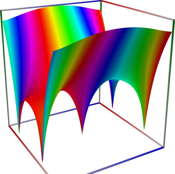

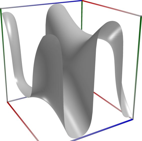
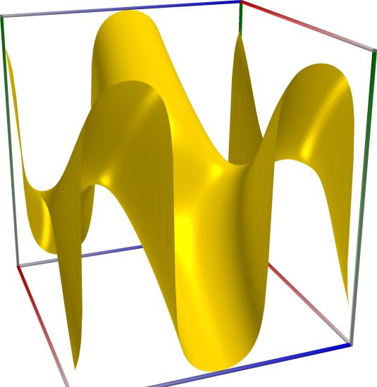
3D wpf plot: real part (left figure), imaginary part (middle figure) and absolute value with color-coded phase (right figure) of the complex sine function \(z = \sin(x + iy)\), with \(-6 \le x \le 6\) (blue axis), \(-6 \le y \le 6\) (red axis), \(-10 \le z \le 10\) (green axis). Function values are loglog-transformed.

An example in Python

>>> from xlcalcnet import ereal
>>> ereal.Si(0.5)
ereal('5.2359877559829887307E-1')
>>> ereal.Si('0.51')
ereal('5.3518479027559984754E-1')

An example with real input:

>>> from xlcalcnet import dec, mpm, gmp, fpm, apm
>>> mpm.dps = 40; x = 3.0
>>> \mathrm{d}x = dec.si(x); mx = mpm.si(x); gx = gmp.si(x)
>>> fx = fpm.si(x); ax = apm.si(x)
>>> mpm.show([\mathrm{d}x, mx, gx, fx, ax])
dec:  1.848652527999468256397730251111973245165E+0
mpm:  1.848652527999468256397730251111973245165e+0
gmp:  1.848652527999468256397730251111973245165E+00
fpm:  1.84865252799947E+00
apm:  1.848652527999468256397730251111973245165e+0 (6.21e-40%)

An example with complex input:

>>> from xlcalcnet import dec, mpm, gmp, fpm, apm
>>> mpm.dps = 20; z = '3.0 + 4.0j'
>>> \mathrm{d}z = dec.si(z); mz = mpm.si(z); gz = gmp.si(z)
>>> fz = fpm.si(z); az = apm.si(z)
>>> mpm.show([\mathrm{d}z, mz, gz, fz, az], aligned=True)
dec: 6.7479950814040320927E+0              - 3.4986637211319094706E+0j
mpm: 6.7479950814040320927e+0              - 3.4986637211319094706e+0j
gmp: 6.7479950814040320927E+00             - 3.4986637211319094706E+00j
fpm: 6.74799508140403E+00                  - 3.49866372113191E+00j
apm: 6.7479950814040320927e+0 (1.004e-19%) - 3.4986637211319094706e+0 (-4.842e-20%)j

Cosine integral \(\mathrm{Ci}(x)\)

ctx.cos_integral(z)

where ctx is math53 or ctxflint.

Returns the cosine integral \(\displaystyle \mathrm{Ci}(x) = -\int_x^{\infty} \frac{\cos(t)}{t} \, \mathrm{d}t = \gamma + \log(x) + \int_0^x \frac{\cos(t) - 1}{t} \, \mathrm{d}t\), and \(\text{Ci}(x) = \text{Ci}(-x)\) for \(x<0\).

For complex \(z\), the cosine integral \(\mathrm{Ci}(z)\), can be computed using

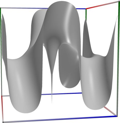
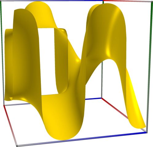
\[\mathrm{Ci}(z) = \log(z) - \frac{1}{2} \left[ e^{iz} U(1,1,-iz) + e^{-iz} U(1,1,iz) + \log(-iz) + \log(iz) \right]\]

See also Wikipedia [1426], MathWorld [1046], NIST [849], Ehrhardt [309] (3.4.2), Flint [839], Flint [832], Mpmath [681].

\(\quad\) \(\quad\)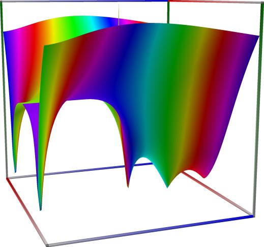

3D wpf plot: real part (left figure), imaginary part (middle figure) and absolute value with color-coded phase (right figure) of the complex sine function \(z = \sin(x + iy)\), with \(-6 \le x \le 6\) (blue axis), \(-6 \le y \le 6\) (red axis), \(-10 \le z \le 10\) (green axis). Function values are loglog-transformed.

An example in Python

>>> from xlcalcnet import ereal
>>> ereal.Ci(0.5)
ereal('5.2359877559829887307E-1')
>>> ereal.Ci('0.51')
ereal('5.3518479027559984754E-1')

An example with real input:

>>> from xlcalcnet import dec, mpm, gmp, fpm, apm
>>> mpm.dps = 40; x = 3.0
>>> \mathrm{d}x = dec.ci(x); mx = mpm.ci(x); gx = gmp.ci(x)
>>> fx = fpm.ci(x); ax = apm.ci(x)
>>> mpm.show([\mathrm{d}x, mx, gx, fx, ax])
dec:  1.196297860080003276264722811766778505468E-1
mpm:  1.196297860080003276264722811766778505468e-1
gmp:  1.196297860080003276264722811766778505468E-01
fpm:  1.19629786008000E-01
apm:  1.196297860080003276264722811766778505468e-1 (1.799e-39%)

An example with complex input:

>>> from xlcalcnet import dec, mpm, gmp, fpm, apm
>>> mpm.dps = 20; z = '3.0 + 4.0j'
>>> \mathrm{d}z = dec.ci(z); mz = mpm.ci(z); gz = gmp.ci(z)
>>> fz = fpm.ci(z); az = apm.ci(z)
>>> mpm.show([\mathrm{d}z, mz, gz, fz, az], aligned=True)
dec: -3.4957570339825683441E+0               - 5.1759052151768084089E+0j
mpm: -3.4957570339825683441e+0               - 5.1759052151768084089e+0j
gmp: -3.4957570339825683441E+00              - 5.1759052151768084089E+00j
fpm: -3.49575703398257E+00                   - 5.17590521517681E+00j
apm: -3.4957570339825683441e+0 (-9.692e-20%) - 5.1759052151768084089e+0 (-6.546e-20%)j