Hurwitz zeta and related functions

Hurwitz zeta function, \(\zeta(s,a)\)

ctx.hurwitz_zeta(s, a)

where ctx is math53, ctxflint.

Returns the Hurwitz zeta function, defined as \(\displaystyle \zeta(s,a) = \sum_{k=0}^\infty \frac{1}{(a+k)^s} \,\), \(s>1, a \ne 0,-1,-2, \ldots\), and by analytic continuation for \(s \ne 0\). The amath implementation requires \(a>0\). If \(a=1\) then \(\zeta(s)\) is returned, and if \(s=0\) the result is \(\frac{1}{2}-a\).

See also Wikipedia [1431], MathWorld [1033], NIST [18], Ehrhardt [309] (3.6.6), Flint [827].

\[\zeta\left(-n,a\right)=-\frac{B_{n+1}\left(a\right)}{n+1}.\]

\[\zeta\left(s,1\right)=\zeta\left(s\right).\]

\[\zeta\left(s,\tfrac{1}{2}\right)=(2^{s}-1)\zeta\left(s\right).\]

\[\zeta'\left(0,a\right)=\log\Gamma\left(a\right)-\tfrac{1}{2}\log\left(2\pi\right).\]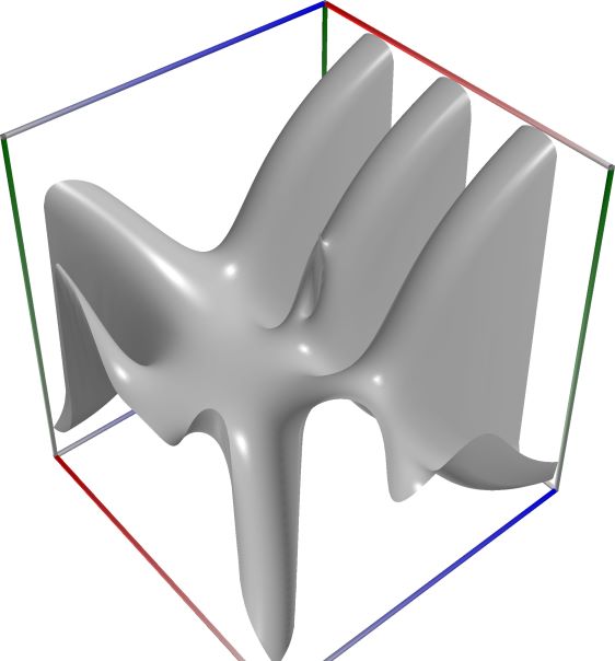

\(\quad\) \(\quad\)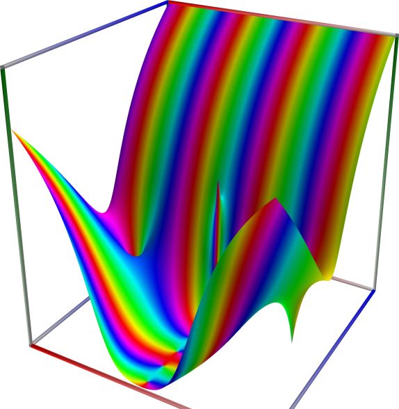

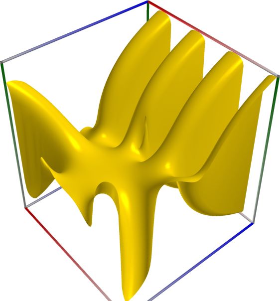
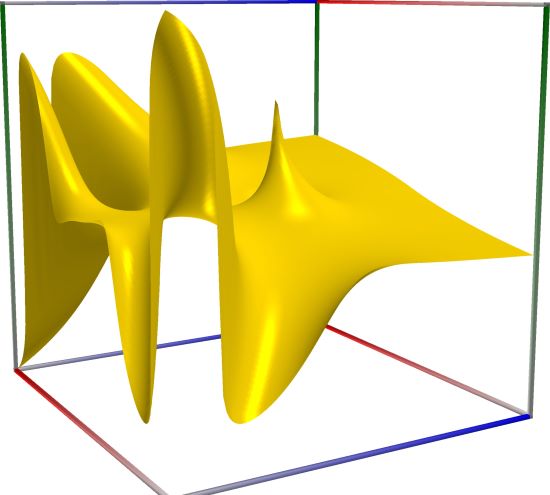
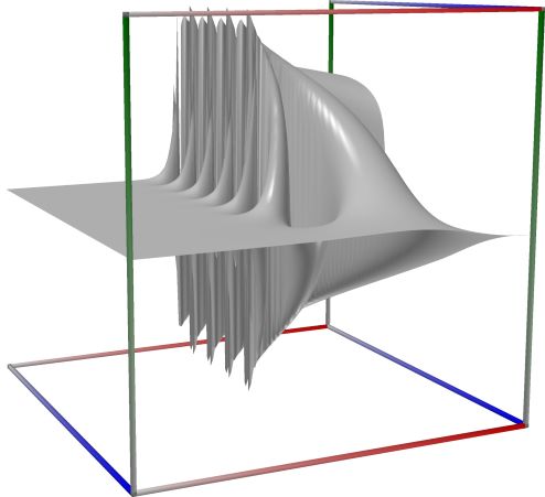
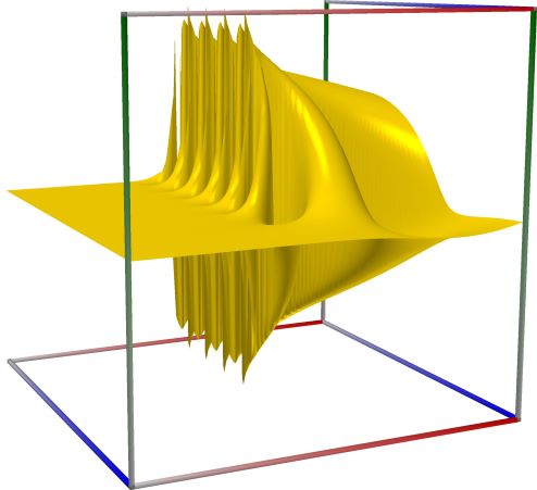
3D wpf plot: real part (left figure), imaginary part (middle figure) and absolute value with color-coded phase (right figure) of the complex sine function \(z = \sin(x + iy)\), with \(-6 \le x \le 6\) (blue axis), \(-6 \le y \le 6\) (red axis), \(-10 \le z \le 10\) (green axis). Function values are loglog-transformed.

\(\quad\) \(\quad\)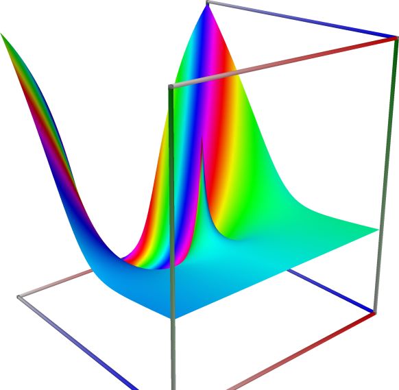

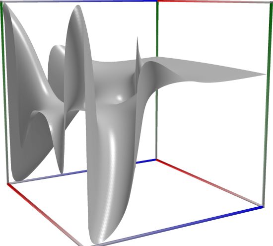
3D wpf plot: real part (left figure), imaginary part (middle figure) and absolute value with color-coded phase (right figure) of the complex sine function \(z = \sin(x + iy)\), with \(-6 \le x \le 6\) (blue axis), \(-6 \le y \le 6\) (red axis), \(-10 \le z \le 10\) (green axis). Function values are loglog-transformed.

\(\quad\) \(\quad\)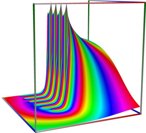

3D wpf plot: real part (left figure), imaginary part (middle figure) and absolute value with color-coded phase (right figure) of the complex sine function \(z = \sin(x + iy)\), with \(-6 \le x \le 6\) (blue axis), \(-6 \le y \le 6\) (red axis), \(-10 \le z \le 10\) (green axis). Function values are loglog-transformed.

An example in Python

>>> from xlcalcnet import ereal
>>> ereal.HurwitzZeta(2,5)
ereal('5.2359877559829887307E-1')
>>> ereal.HurwitzZeta(2,'51')
ereal('5.3518479027559984754E-1')

An example with real input:

>>> from xlcalcnet import dec, mpm, gmp, fpm, apm
>>> mpm.dps = 40; s = '10'; a = '1.5'
>>> \mathrm{d}x = dec.hurwitz(s, a); mx = mpm.hurwitz(s, a); gx = gmp.hurwitz(s, a)
>>> fx = fpm.hurwitz(s, a); ax = apm.hurwitz(s, a)
>>> mpm.show([\mathrm{d}x, mx, gx, fx, ax])
dec:  1.745035575790129990031595502635439715798E-2
mpm:  1.745035575790129990031595502635439715798e-2
gmp:  1.745035575790129990031595502635439715798E-02
fpm:  1.74503557579013E-02
apm:  1.745035575790129990031595502635439715798e-2 (1.028e-39%)

An example with complex input:

>>> from xlcalcnet import dec, mpm, gmp, fpm, apm
>>> mpm.dps = 20; s = '10 + 5j'; a = '5.0 + 3j'
>>> \mathrm{d}z = dec.hurwitz(s, a); mz = mpm.hurwitz(s, a); gz = gmp.hurwitz(s, a)
>>> fz = fpm.hurwitz(s, a); az = apm.hurwitz(s, a)
>>> mpm.show([\mathrm{d}z, mz, gz, fz, az],  aligned=True)
dec: -2.9834537360028672178E-8               - 3.9761878565611985695E-7j
mpm: -2.9834537360028672178e-8               - 3.9761878565611985695e-7j
gmp: -2.9834537360028672178E-08              - 3.9761878565611985695E-07j
fpm: -2.98345373600287E-08                   - 3.97618785656120E-07j
apm: -2.9834537360028672177e-8 (-8.461e-20%) - 3.9761878565611985695e-7 (-5.079e-20%)j

Generalized harmonic number function, \(H_x^{(r)}\)

math53.harmonic2(x, s)

Returns the generalized harmonic function \(H_x^{(r)} = \zeta(r) - \zeta(r,x+1)\) for \(r \ne 1\) and \(H_x^{(r)} = H_x\) for \(r = 1\).

See also: Wikipedia [1390], MathWorld [995], Ehrhardt [309] (3.6.21).

An example in Python

>>> from xlcalcnet import ereal
>>> ereal.Harmonic2(5, 10.5)
ereal('5.2359877559829887307E-1')
>>> ereal.Harmonic2(5, '10.1')
ereal('5.3518479027559984754E-1')

An example with real input:

>>> from xlcalcnet import dec, mpm, gmp, fpm, apm
>>> mpm.dps = 40; x = '10'; r = '1.5'
>>> \mathrm{d}x = dec.harmonic2(x, r); mx = mpm.harmonic2(x, r); gx = gmp.harmonic2(x, r)
>>> fx = fpm.harmonic2(x, r); ax = apm.harmonic2(x, r)
>>> mpm.show([\mathrm{d}x, mx, gx, fx, ax])
dec:  1.995336493345601714521693592714339476261E+0
mpm:  1.995336493345601714521693592714339476261e+0
gmp:  1.995336493345601714521693592714339476261E+00
fpm:  1.99533649334560E+00
apm:  1.995336493345601714521693592714339476261e+0 (1.668e-38%)

An example with complex input:

>>> from xlcalcnet import dec, mpm, gmp, fpm, apm
>>> mpm.dps = 20; z = '10 + 5j'; r = '5.0 + 3j'
>>> \mathrm{d}z = dec.harmonic2(z, r); mz = mpm.harmonic2(z, r); gz = gmp.harmonic2(z, r)
>>> fz = fpm.harmonic2(z, r); az = apm.harmonic2(z, r)
>>> mpm.show([\mathrm{d}z, mz, gz, fz, az],  aligned=True)
dec: 9.8046716104400925422E-1              - 2.5426375920749034566E-2j
mpm: 9.8046716104400925422e-1              - 2.5426375920749034566e-2j
gmp: 9.8046716104400925422E-01             - 2.5426375920749034566E-02j
fpm: 9.80467161044009E-01                  - 2.54263759207490E-02j
apm: 9.8046716104400925422e-1 (8.639e-20%) - 2.5426375920749034566e-2 (-1.041e-19%)j

Bernoulli numbers, \(B_n\)

ctx.bernoulli(n)

where ctx is math53, ctxboost or ctxflint.

Note ctxboost.BernoulliB2n(n)

Returns the Bernoulli numbers \(B_n\), which are defined by their generating function \(\displaystyle \frac{1}{e^t-1} \sum_{n=0}^{\infty} B_n \frac{t^n}{n!}\), \(|t < 2\pi|\). If \(n<0\) or if \(n>2\) is odd, the result is \(0\), and \(B_1=-1/2\).

See also Wikipedia [1354], MathWorld [949], NIST [249], BoostMath [99], Ehrhardt [309] (3.10.2), Mpmath [608].

An example in Python

>>> from xlcalcnet import ereal
>>> ereal.Bernoulli(8)
ereal('5.2359877559829887307E-1')
>>> ereal.Bernoulli(14)
ereal('5.3518479027559984754E-1')

An example:

>>> from xlcalcnet import dec, mpm, gmp, fpm, apm
>>> mpm.dps = 40; n = '16'
>>> \mathrm{d}x = dec.bernoulli(n); mx = mpm.bernoulli(n); gx = gmp.bernoulli(n)
>>> fx = fpm.bernoulli(n); ax = apm.bernoulli(n)
>>> mpm.show([\mathrm{d}x, mx, gx, fx, ax])
dec:  -7.092156862745098039215686274509803921569E+0
mpm:  -7.092156862745098039215686274509803921569e+0
gmp:  -7.092156862745098039215686274509803921569E+00
fpm:  -7.09215686274510E+00
apm:  -7.092156862745098039215686274509803921569e+0 (-1.295e-39%)

Bernoulli polynomials, \(B_n(x)\)

math53.bernpoly(n, x)

Returns \(\displaystyle B_n(x) = \sum_{n=0}^{\infty} \binom{n}{k} B_k x^{n-k}\), the Bernoulli polynomial of degree \(n \ge 0\).

See also Wikipedia [1355], MathWorld [950], NIST [249], Ehrhardt [309] (3.10.3), Flint [792], Mpmath [610].

See the Amath documentation (p. 146) for connection formula to Hurwitz Zeta.

An example in Python

>>> from xlcalcnet import ereal
>>> ereal.Bernpoly(3,4)
ereal('5.2359877559829887307E-1')
>>> ereal.Bernpoly(13,14)
ereal('5.3518479027559984754E-1')

An example with real input:

>>> from xlcalcnet import dec, mpm, gmp, fpm, apm
>>> mpm.dps = 40; n = '16'; x = '1.5'
>>> \mathrm{d}x = dec.bernpoly(n, x); mx = mpm.bernpoly(n, x); gx = gmp.bernpoly(n, x)
>>> fx = fpm.bernpoly(n, x); ax = apm.bernpoly(n, x)
>>> mpm.show([\mathrm{d}x, mx, gx, fx, ax])
dec:  7.092428708543964460784313725490196078431E+0
mpm:  7.092428708543964460784313725490196078431e+0
gmp:  7.092428708543964460784313725490196078431E+00
fpm:  7.09242870854397E+00
apm:  7.092428708543964460784313725490196078432e+0 (1.457e-37%)

An example with complex input:

>>> from xlcalcnet import dec, mpm, gmp, fpm, apm
>>> mpm.dps = 20; n = '16'; z = '10 + 5j'
>>> \mathrm{d}z = dec.bernpoly(n, z); mz = mpm.bernpoly(n, z); gz = gmp.bernpoly(n, z)
>>> fz = fpm.bernpoly(n, z); az = apm.bernpoly(n, z)
>>> mpm.show([\mathrm{d}z, mz, gz, fz, az],  aligned=True)
dec: 9.1935042603632624118E+14              + 2.9617209867479000000E+16j
mpm: 9.1935042603632624118e+14              + 2.9617209867479000000e+16j
gmp: 9.1935042603632624118E+14              + 2.9617209867479000000E+16j
fpm: 9.19350426036326E+14                   + 2.96172098674790E+16j
apm: 9.1935042603632624118e+14 (1.089e-18%) + 2.9617209867479000000e+16 (1.03e-19%)j

Euler numbers

ctx.eulernum(n)

where ctx is math53, ctxflint.

Returns the Euler numbers \(E_n\). See also Wikipedia [1383], MathWorld [992], Flint [826], Ehrhardt [309] (3.10.8), Mpmath [637].

The Euler numbers \(E_n\) can be defined as

\[E_n = \frac{4^n \beta(n+1)}{\zeta(n)} \frac{2B_n}{\pi}\]

An example:

>>> from xlcalcnet import dec, mpm, gmp, fpm, apm
>>> mpm.dps = 40; n = '16'
>>> \mathrm{d}x = dec.eulernum(n); mx = mpm.eulernum(n); gx = gmp.eulernum(n)
>>> fx = fpm.eulernum(n); ax = apm.eulernum(n)
>>> mpm.show([\mathrm{d}x, mx, gx, fx, ax])
dec:  1.939151214500000000000000000000000000000E+10
mpm:  1.939151214500000000000000000000000000000e+10
gmp:  1.939151214500000000000000000000000000000E+10
fpm:  1.93915121450000E+10
apm:  1.939151214500000000000000000000000000000e+10 (0.0%)

Euler polynomials, \(E_n(x)\)

math53.eulerpoly(n, x)

Returns \(\displaystyle E_n(x) = \frac{2}{n+1} \left( B_{n+1}(x)-2^{n+1}B_{n+1}\left(\frac{x}{2}\right) \right)\), the Euler polynomial of degree \(n \ge 0\). Special values include the Euler numbers \(E_n = 2^n E_n(1/2)\).

See also Wikipedia [1384], MathWorld [993], NIST [249], Ehrhardt [309] (3.10.9), Mpmath [638].

\[E_{n-1}\left(x\right)=\frac{2}{n}\left(B_{n}\left(x\right)-2^{n}B_{n}\left(\tfrac{1}{2}x\right)\right),\]

\[E_{n-1}\left(x\right)=\frac{2^{n}}{n}\left(B_{n}\left(\tfrac{1}{2}x+\tfrac{1}{2}\right)-B_{n}\left(\tfrac{1}{2}x\right)\right).\]

An example in Python

>>> from xlcalcnet import ereal
>>> ereal.Eulerpoly(3, 4)
ereal('5.2359877559829887307E-1')
>>> ereal.Eulerpoly(3, 12)
ereal('5.3518479027559984754E-1')

An example with real input:

>>> from xlcalcnet import dec, mpm, gmp, fpm, apm
>>> mpm.dps = 40; n = '16'; x = '1.5'
>>> \mathrm{d}x = dec.eulerpoly(n, x); mx = mpm.eulerpoly(n, x); gx = gmp.eulerpoly(n, x)
>>> fx = fpm.eulerpoly(n, x); ax = apm.eulerpoly(n, x)
>>> mpm.show([\mathrm{d}x, mx, gx, fx, ax])
dec:  -2.958909933929443359375000000000000000000E+5
mpm:  -2.958909933929443359375000000000000000000e+5
gmp:  -2.958909933929443359375000000000000000000E+05
fpm:  -2.95890993392944E+05
apm:  -2.958909933929443359375000000000000000000e+5 (-3.254e-38%)

An example with complex input:

>>> from xlcalcnet import dec, mpm, gmp, fpm, apm
>>> mpm.dps = 20; n = '16'; z = '10 + 5j'
>>> \mathrm{d}z = dec.eulerpoly(n, z); mz = mpm.eulerpoly(n, z); gz = gmp.eulerpoly(n, z)
>>> fz = fpm.eulerpoly(n, z); az = apm.eulerpoly(n, z)
>>> mpm.show([\mathrm{d}z, mz, gz, fz, az],  aligned=True)
dec: -2.7730057139461850000E+15               + 2.6625051419981595000E+16j
mpm: -2.7730057139461850000e+15               + 2.6625051419981595000e+16j
gmp: -2.7730057139461850000E+15               + 2.6625051419981595000E+16j
fpm: -2.77300571394618E+15                    + 2.66250514199816E+16j
apm: -2.7730057139461850000e+15 (-6.053e-18%) + 2.6625051419981595000e+16 (7.45e-19%)j

Barnes G-function

ctxflint.barnes_g(z)

Returns the Barnes G-function of z. See also Wikipedia [1402], MathWorld [987], NIST [22], Whittaker and Watson [1171], Mpmath [656].

Evaluates the Barnes G-function, which generalizes the superfactorial (superfac()) and by extension also the hyperfactorial (hyperfac()) to the complex numbers in an analogous way to how the gamma function generalizes the ordinary factorial.

The Barnes G-function may be defined in terms of a Weierstrass product:

\[G(z+1) = (2\pi)^{z/2} e^{-[z(z+1)+\gamma z^2]/2} \prod_{n=1}^\infty \left[\left(1+\frac{z}{n}\right)^ne^{-z+z^2/(2n)}\right]\]

For positive integers \(n\), we have have relation to superfactorials \(G(n) = \mathrm{sf}(n-2) = 0! \cdot 1! \cdots (n-2)!\).

An example with real input:

>>> from xlcalcnet import dec, mpm, gmp, fpm, apm
>>> mpm.dps = 40; x = '1.5'
>>> \mathrm{d}x = dec.barnesg(x); mx = mpm.barnesg(x); gx = gmp.barnesg(x)
>>> fx = fpm.barnesg(x); ax = apm.barnesg(x)
>>> mpm.show([\mathrm{d}x, mx, gx, fx, ax])
dec:  1.069222649266412949543008878697891604653E+0
mpm:  1.069222649266412949543008878697891604653e+0
gmp:  1.069222649266412949543008878697891604653E+00
fpm:  1.06922264926641E+00
apm:  1.069222649266412949543008878697891604653e+0 (2.147e-39%)

An example with complex input:

>>> from xlcalcnet import dec, mpm, gmp, fpm, apm
>>> mpm.dps = 20; z = '10 + 5j'
>>> \mathrm{d}z = dec.barnesg(z); mz = mpm.barnesg(z); gz = gmp.barnesg(z)
>>> fz = fpm.barnesg(z); az = apm.barnesg(z)
>>> mpm.show([\mathrm{d}z, mz, gz, fz, az],  aligned=True)
dec: 4.0615260490805827996E+3              - 1.5756073051910381056E+3j
mpm: 4.0615260490805827996e+3              - 1.5756073051910381056e+3j
gmp: 4.0615260490805827996E+03             - 1.5756073051910381056E+03j
fpm: 4.06152604908058E+03                  - 1.57560730519104E+03j
apm: 4.0615260490805827996e+3 (8.969e-19%) - 1.5756073051910381056e+3 (-2.808e-18%)j

Logarithm of Barnes G function

ctx.logbarnes_g(x)

where ctx is math53 or ctxflint.

Returns \(\log G(z)\), the logarithm of Barnes \(G\) function, with log G(z) = (z-1) log Gamma(z) - zeta’(-1,z) + zeta’(-1).

See also: Wikipedia [1402], MathWorld [987], MathWorld [1003], NIST [22], Ehrhardt [309] (3.5.6.9).

Computes Barnes G-function or the logarithmic Barnes G-function, respectively. The logarithmic version has branch cuts on the negative real axis and is continuous elsewhere in the complex plane, in analogy with the logarithmic gamma function. The functional equation

\[\log G(z+1) = \log \Gamma(z) + \log G(z).\]

holds for all z.

An example in Python

>>> from xlcalcnet import ereal
>>> ereal.LogBarnesG(7.1)
ereal('5.2359877559829887307E-1')
>>> ereal.LogBarnesG('4.51')
ereal('5.3518479027559984754E-1')

An example with real input:

>>> from xlcalcnet import dec, mpm, gmp, fpm, apm
>>> mpm.dps = 40; x = '1.5'
>>> \mathrm{d}x = dec.Logbarnesg(x); mx = mpm.Logbarnesg(x); gx = gmp.Logbarnesg(x)
>>> fx = fpm.Logbarnesg(x); ax = apm.Logbarnesg(x)
>>> mpm.show([\mathrm{d}x, mx, gx, fx, ax])
dec:  6.693188843500470427402868586818440410225E-2
mpm:  6.693188843500470427402868586818440410225e-2
gmp:  6.693188843500470427402868586818440410225E-02
fpm:  6.69318884350047E-02
apm:  6.693188843500470427402868586818440410225e-2 (2.144e-39%)

An example with complex input:

>>> from xlcalcnet import dec, mpm, gmp, fpm, apm
>>> mpm.dps = 20; z = '10 + 5j'
>>> \mathrm{d}z = dec.Logbarnesg(z); mz = mpm.Logbarnesg(z); gz = gmp.Logbarnesg(z)
>>> fz = fpm.Logbarnesg(z); az = apm.Logbarnesg(z)
>>> mpm.show([\mathrm{d}z, mz, gz, fz, az],  aligned=True)
dec: 8.3794095077852315352E+0              - 3.7006227106476637064E-1j
mpm: 8.3794095077852315352e+0              - 3.7006227106476637064e-1j
gmp: 8.3794095077852315352E+00             - 3.7006227106476637064E-01j
fpm: 8.37940950778523E+00                  - 3.70062271064766E-01j
apm: 8.3794095077852315352e+0 (1.617e-19%) + 5.6178605493551511922e+1 (4.825e-20%)j

Hyperfactorial

ctxflint.hyperfactorial(z)

Returns the hyperfactorial of z. See also Wikipedia [1391], MathWorld [998], of Integer Sequences [450], Mpmath [663].

Computes the hyperfactorial, defined for integers as the product

\[H(n) = \prod_{k=1}^n k^k.\]

The hyperfactorial satisfies the recurrence formula \(H(z) = z^z H(z-1)\). It can be defined more generally in terms of the Barnes G-function (see barnesg()) and the gamma function by the formula

\[H(z) = \frac{\Gamma(z+1)^z}{G(z+1)}.\]

An example with real input:

>>> from xlcalcnet import dec, mpm, gmp, fpm, apm
>>> mpm.dps = 40; x = '1.5'
>>> \mathrm{d}x = dec.hyperfac(x); mx = mpm.hyperfac(x); gx = gmp.hyperfac(x)
>>> fx = fpm.hyperfac(x); ax = apm.hyperfac(x)
>>> mpm.show([\mathrm{d}x, mx, gx, fx, ax])
dec:  1.617488527948946062817035460231792759012E+0
mpm:  1.617488527948946062817035460231792759012e+0
gmp:  1.617488527948946062817035460231792759012E+00
fpm:  1.61748852794895E+00
apm:  1.617488527948946062817035460231792771778e+0 (2.059e-33%)

An example with complex input:

>>> from xlcalcnet import dec, mpm, gmp, fpm, apm
>>> mpm.dps = 20; z = '10.5 + 1j'
>>> \mathrm{d}z = dec.hyperfac(z); mz = mpm.hyperfac(z); gz = gmp.hyperfac(z)
>>> fz = fpm.hyperfac(z); az = apm.hyperfac(z)
>>> mpm.show([\mathrm{d}z, mz, gz, fz, az],  aligned=True)
dec: 4.6669290555030590228E+48              + 1.2961711093304818907E+49j
mpm: 4.6669290555030590228e+48              + 1.2961711093304818907e+49j
gmp: 4.6669290555030590228E+48              + 1.2961711093304818907E+49j
fpm: 4.66692905550306E+48                   + 1.29617110933048E+49j
apm: 4.6669290555030590228e+48 (5.257e-17%) + 1.2961711093304818907e+49 (3.064e-17%)j

Superfactorial

ctxflint.superfactorial(z)

Returns the Superfactorial of z. See also Wikipedia [1398], MathWorld [1009], of Integer Sequences [451], Mpmath [668].

Computes the superfactorial, defined as the product of consecutive factorials

\[\mathrm{sf}(n) = \prod_{k=1}^n k!\]

For general complex \(z\), \(\mathrm{sf}(z)\) is defined in terms of the Barnes G-function (see barnesg()).

\[\mathrm{sf}(z) = G(z+2)\]

An example with real input:

>>> from xlcalcnet import dec, mpm, gmp, fpm, apm
>>> mpm.dps = 40; x = '1.5'
>>> \mathrm{d}x = dec.superfac(x); mx = mpm.superfac(x); gx = gmp.superfac(x)
>>> fx = fpm.superfac(x); ax = apm.superfac(x)
>>> mpm.show([\mathrm{d}x, mx, gx, fx, ax])
dec:  1.259648257495192144086307951096069825563E+0
mpm:  1.259648257495192144086307951096069825563e+0
gmp:  1.259648257495192144086307951096069825563E+00
fpm:  1.25964825749519E+00
apm:  1.259648257495192144086307951096069825563e+0 (9.113e-40%)

An example with complex input:

>>> from xlcalcnet import dec, mpm, gmp, fpm, apm
>>> mpm.dps = 20; z = '10.5 + 1j'
>>> \mathrm{d}z = dec.superfac(z); mz = mpm.superfac(z); gz = gmp.superfac(z)
>>> fz = fpm.superfac(z); az = apm.superfac(z)
>>> mpm.show([\mathrm{d}z, mz, gz, fz, az],  aligned=True)
dec: 1.8638249390462723001E+30             - 8.9432323302755030353E+30j
mpm: 1.8638249390462723001e+30             - 8.9432323302755030353e+30j
gmp: 1.8638249390462723001E+30             - 8.9432323302755030353E+30j
fpm: 1.86382493904627E+30                  - 8.94323233027550E+30j
apm: 1.8638249390462723001e+30 (2.42e-18%) - 8.9432323302755030353e+30 (-1.345e-18%)j