Introduction to 2D functions plots#
Plots of continuous distribution functions#
Some text
Probability density function (pdf)#
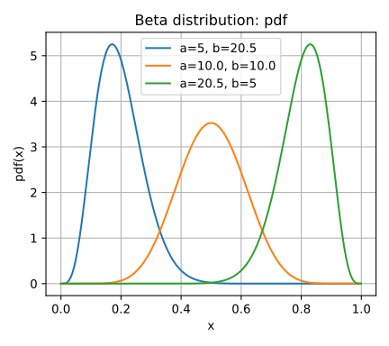
The Python code for the example below can be found online in the DataXlCalcNet repository or in the corresponding local DataXlCalcNet folder in the file D07_DistPlotContinuous.py, and the XML code in the file D07_DistPlotContinuous.2D.xml.
To produce the figure as shown below, the try-block at the end of the file should look like this:
try:
    if __name__ == '__main__':
        ylim = None
        target = 'pdf' # pdf, cdf, 'sf', 'hf', 'chf', 'qtf', 'isf'

        Title = 'Beta distribution'
        a = [5, 10.0, 20.5]
        b = [20.5, 10.0, 5]
        xlim = [0, 0.999]
        if target=='hf': ylim=[0, 100]

        dlist = []
        ltext = []
        for j in range(len(a)):
            dlist.append(dreal.dist_beta(a[j], b[j]))
            ltext.append('a=' + str(a[j]) + ', b=' + str(b[j]))

        DistPlotContinuous(Title = Title, dlist=dlist, xlim = xlim,
            ylim = ylim, target = target, ltext = ltext, marker='o',
            markersize=0)
Cumulative distribution function (cdf)#
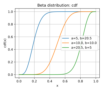
The Python code for the example below can be found online in the DataXlCalcNet repository or in the corresponding local DataXlCalcNet folder in the file D07_DistPlotContinuous.py, and the XML code in the file D07_DistPlotContinuous.2D.xml.
To produce the figure as shown below, the try-block at the end of the file should look like this:
try:
    if __name__ == '__main__':
        ylim = None
        target = 'cdf' # pdf, cdf, 'sf', 'hf', 'chf', 'qtf', 'isf'

        Title = 'Beta distribution'
        a = [5, 10.0, 20.5]
        b = [20.5, 10.0, 5]
        xlim = [0, 0.999]
        if target=='hf': ylim=[0, 100]

        dlist = []
        ltext = []
        for j in range(len(a)):
            dlist.append(dreal.dist_beta(a[j], b[j]))
            ltext.append('a=' + str(a[j]) + ', b=' + str(b[j]))

        DistPlotContinuous(Title = Title, dlist=dlist, xlim = xlim,
            ylim = ylim, target = target, ltext = ltext, marker='o',
            markersize=0)
Plots of discrete distribution functions#
Probability mass function (pmf)#
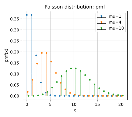
The Python code for the example below can be found online in the DataXlCalcNet repository or in the corresponding local DataXlCalcNet folder in the file D08_DistPlotDiscrete.py, and the XML code in the file D08_DistPlotDiscrete.2D.xml.
To produce the figure as shown below, the try-block at the end of the file should look like this:
try:
    if __name__ == '__main__':
        ylim = None

        Title = 'Poisson distribution'
        target = 'pmf' # pmf, cdf, 'sf', 'hf', 'chf', 'qtf', 'isf'
        mu = [1, 4, 10]
        xlim = [0.0, 20.0]
        ylim = None
        if target=='qtf': ylim=[0, 20]

        dlist = []
        ltext = []
        for j in range(len(mu)):
            dlist.append(dreal.dist_poisson(mu[j]))
            ltext.append('mu=' + str(mu[j]))
        DistPlotDiscrete(Title = Title, dlist=dlist, xlim = xlim,  ylim = ylim,
            target = target, ltext = ltext, lattice=True, marker='o',
            markersize=3, vertical_lines=True)
Cumulative distribution function (cdf)#
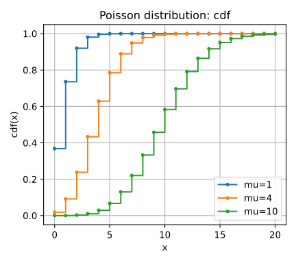
The Python code for the example below can be found online in the DataXlCalcNet repository or in the corresponding local DataXlCalcNet folder in the file D08_DistPlotDiscrete.py, and the XML code in the file D08_DistPlotDiscrete.2D.xml.
To produce the figure as shown below, the try-block at the end of the file should look like this:
try:
    if __name__ == '__main__':
        ylim = None

        Title = 'Poisson distribution'
        target = 'cdf' # pmf, cdf, 'sf', 'hf', 'chf', 'qtf', 'isf'
        mu = [1, 4, 10]
        xlim = [0.0, 20.0]
        ylim = None
        if target=='qtf': ylim=[0, 20]

        dlist = []
        ltext = []
        for j in range(len(mu)):
            dlist.append(dreal.dist_poisson(mu[j]))
            ltext.append('mu=' + str(mu[j]))
        DistPlotDiscrete(Title = Title, dlist=dlist, xlim = xlim,  ylim = ylim,
            target = target, ltext = ltext, lattice=True, marker='o',
            markersize=3, vertical_lines=True)