Functions with real input and complex results

Expj (Cis) function

The XML code for the example below can be found online in the DataXlCalcNet repository or in the corresponding local DataXlCalcNet folder in the files D01a_Path_Func_Expj_2Dx.3D.xml (D01a-e).

Returns \(e^{iz} = \cos(z) + i \sin(z)\). See also Wikipedia [1376], MathWorld [1021].

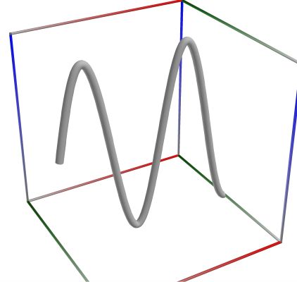
The example below uses the following code in C#, for real part only

var y = Math.Sin(t);
var x = t;
var z = 0;

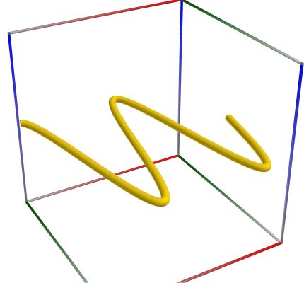
The example below uses the following code in C#, for imaginary part only

var z = -Math.Cos(t);
var x = t;
var y = 0;

The example below uses the following code in C#, for real and imaginary part combined

var x = Math.Sin(t);
var y = -Math.Cos(t);
var z = t;

Some text

\(\quad\) \(\quad\)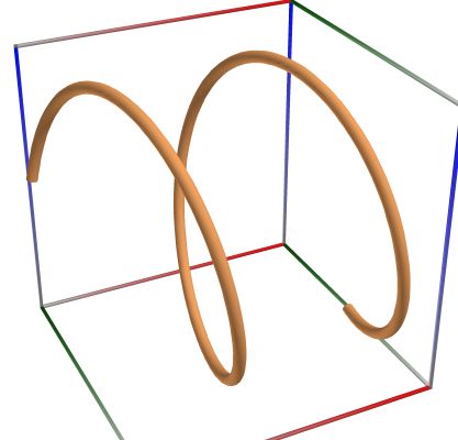

Left figure: Expj (Cis) function, real part only. Orthographic camera.

Middle figure: Expj (Cis) function, imaginary part only. Orthographic camera.

Right figure: Expj (Cis) function as full 3D curve. Orthographic camera.

\(\quad\)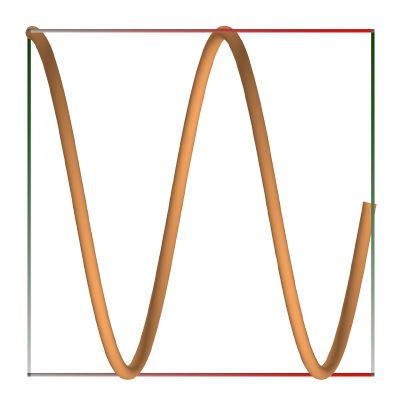

Hankel function of the first kind \(H_{1, \nu}(x)\)

The XML code for the example below can be found online in the DataXlCalcNet repository or in the corresponding local DataXlCalcNet folder in the files D02a_Path_Func_Hankel1_2Dx.3D.xml (D02a-c).

Returns the Hankel function of the first kind, defined as \(\displaystyle H^{(1)}_{\nu}(x) = J_{\nu}(x) + i Y_{\nu}(x)\).

See also Wikipedia [1308], MathWorld [942], NIST [444], BoostMath [115].

The example below uses the following code in C#, for real part only

var y = ctx.bessel_j0(t);
var x = t;
var z = 0;

The example below uses the following code in C#, for imaginary part only

var z = -ctx.bessel_y0(t);
var x = t;
var y = 0;

The example below uses the following code in C#, for real and imaginary part combined

var z = ctx.bessel_j0(t);
var y = -ctx.bessel_y0(t);
var x = t;

\(\quad\) \(\quad\)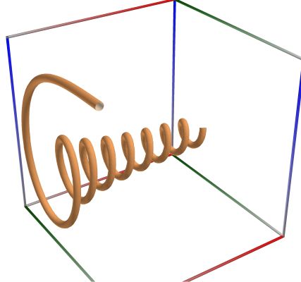

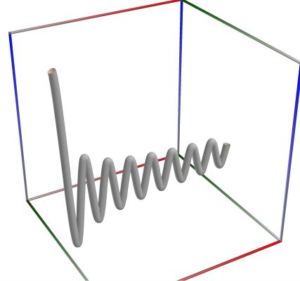
Left figure: Hankel function of the first kind \(H_{1, \nu}(x)\), real part only. Orthographic camera.

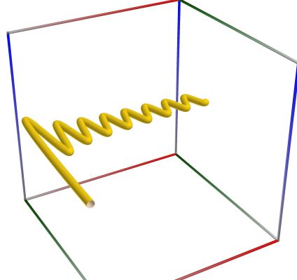
Middle figure: Hankel function of the first kind \(H_{1, \nu}(x)\), imaginary part only. Orthographic camera.

Right figure: Hankel function of the first kind \(H_{1, \nu}(x)\), as full 3D curve. Orthographic camera.

Hankel function of the second kind \(H_{2, \nu}(x)\)

The XML code for the example below can be found online in the DataXlCalcNet repository or in the corresponding local DataXlCalcNet folder in the files D03a_Path_Func_Hankel2_2Dx.3D.xml (D03a-c).

Returns the Hankel function of the second kind, defined as \(\displaystyle H^{(2)}_{\nu}(x) = J_{\nu}(x) - i Y_{\nu}(x)\).

See also Wikipedia [1308], MathWorld [943], NIST [444], BoostMath [115].

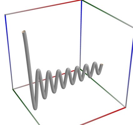
The example below uses the following code in C#, for real part only

var y = ctx.bessel_j0(t);
var x = t;
var z = 0;

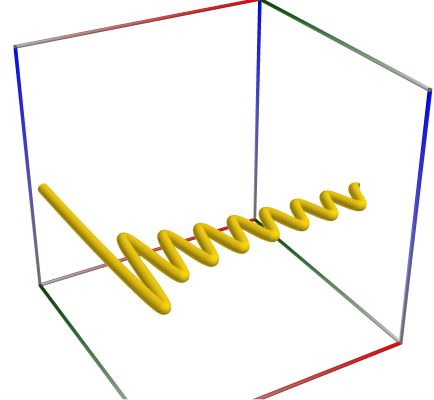
The example below uses the following code in C#, for imaginary part only

var z = ctx.bessel_y0(t);
var x = t;
var y = 0;

The example below uses the following code in C#, for real and imaginary part combined

var z = ctx.bessel_j0(t);
var y = ctx.bessel_y0(t);
var x = t;

\(\quad\) \(\quad\)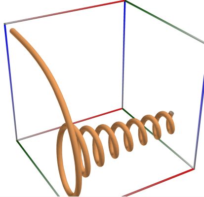

Left figure: Hankel function of the second kind \(H_{2, \nu}(x)\), real part only. Orthographic camera.

Middle figure: Hankel function of the second kind \(H_{2, \nu}(x)\), imaginary part only. Orthographic camera.

Right figure: Hankel function of the second kind \(H_{2, \nu}(x)\), as full 3D curve. Orthographic camera.

Kelvin functions ber and bei

The XML code for the example below can be found online in the DataXlCalcNet repository or in the corresponding local DataXlCalcNet folder in the files D04a_Path_Func_KelvinBerBei_2Dx.3D.xml (D04a-c).

Returns the Kelvin functions ber bei. See also Wikipedia [1383], MathWorld [1024], NIST [445].

The following conventions are used as in Maple (with \(a = \sqrt{2}/2\)):

\[\text{ber}(\nu, x) + i \text{bei}(\nu, x) = J_{\nu}(x(-a + i a))\]

\[\text{ber}(\nu, x) - i \text{bei}(\nu, x) = J_{\nu}(x(-a - i a))\]

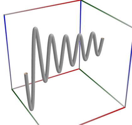
The example below uses the following code in C#, for the real part only

var a = ctx.exp(t / ctx.sqrt(2));
var x = t;
var y = 0;
var z = ctx.kelvin_ber(1,t) / a;

The example below uses the following code in C#, for the imaginary part only

var a = ctx.exp(t / ctx.sqrt(2));
var x = t;
var y = ctx.kelvin_bei(1,t) / a;
var z = 0;

The example below uses the following code in C#, for the real and imaginary parts combined

var a = ctx.exp(t / ctx.sqrt(2));
var x = t;
var y = ctx.kelvin_bei(1,t) / a;
var z = ctx.kelvin_ber(1,t) / a;

\(\quad\) \(\quad\)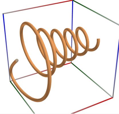

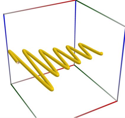
Left figure: Kelvin functions ber. Orthographic camera.

Middle figure: Kelvin function bei. Orthographic camera.

Right figure: Kelvin functions ber and bei, as full 3D curve. Orthographic camera.

Kelvin functions ker and kei

The XML code for the example below can be found online in the DataXlCalcNet repository or in the corresponding local DataXlCalcNet folder in the files D05a_Path_Func_KelvinKerKei_2Dx.3D.xml (D05a-c).

Returns the Kelvin function ker. See also Wikipedia [1385], MathWorld [1026], NIST [445].

The following conventions are used as in Maple (with \(a = \sqrt{2}/2\)):

\[\text{ker}(\nu, x) + i \text{kei}(\nu, x) = e^{-i \nu \pi/2} K_{\nu}(x(a + i a))\]

\[\text{ker}(\nu, x) - i \text{kei}(\nu, x) = e^{i \nu \pi/2} K_{\nu}(x(a - i a))\]

The example below uses the following code in C#, for real part only

var a = ctx.exp(t / ctx.sqrt(2));
var x = t;
var y = 0;
var z = ctx.kelvin_ker(0,t) * a;

The example below uses the following code in C#, for imaginary part only

var a = ctx.exp(t / ctx.sqrt(2));
var x = t;
var y = ctx.kelvin_kei(0,t) * a;
var z = 0;

The example below uses the following code in C#, for real and imaginary part combined

var a = ctx.exp(t / ctx.sqrt(2));
var x = t;
var y = ctx.kelvin_kei(0,t) * a;
var z = ctx.kelvin_ker(0,t) * a;

\(\quad\) \(\quad\)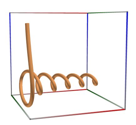

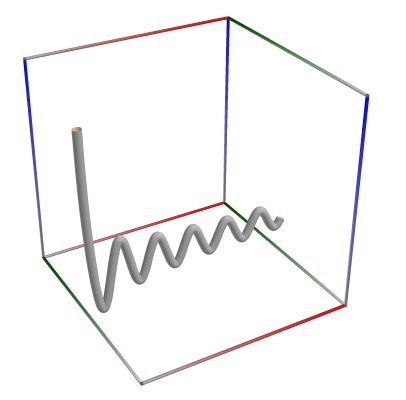
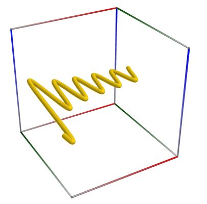
Left figure: Kelvin functions ker. Orthographic camera.

Middle figure: Kelvin function kei. Orthographic camera.

Right figure: Kelvin functions ker and kei, as full 3D curve. Orthographic camera.