Riemann zeta function, and related functions

Riemann zeta function, \(\zeta(s)\)

ctx.zeta(s)

where ctx is math53, mathc53, ctxboost ctxflint.

Returns the Riemann zeta function, defined as \(\displaystyle \zeta(s) = \sum_{k=1}^{\infty} \frac{1}{k^s}\) for \(s>1\), and by analytic continuation for \(s \ne 1\).

See also Wikipedia [1440], MathWorld [1044], NIST [20], BoostMath [165], Ehrhardt [309] (3.6.1.1), Ehrhardt [309] (4.2.63), Flint [829], Mpmath [693].

\(\quad\) \(\quad\)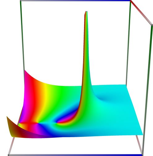

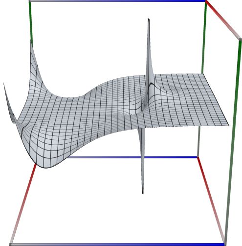
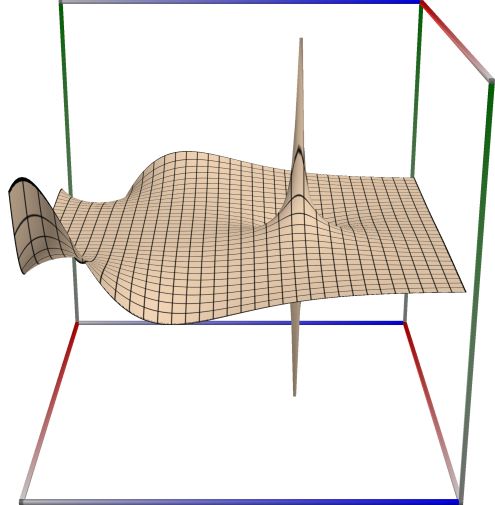
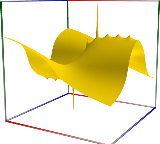
3D wpf plot: real part (left figure), imaginary part (middle figure) and absolute value with color-coded phase (right figure) of the complex sine function \(z = \sin(x + iy)\), with \(-6 \le x \le 6\) (blue axis), \(-6 \le y \le 6\) (red axis), \(-10 \le z \le 10\) (green axis). Function values are loglog-transformed.

An example in Python

>>> from xlcalcnet import ereal
>>> ereal.Zeta(1.5)
ereal('5.2359877559829887307E-1')
>>> ereal.Zeta('1.51')
ereal('5.3518479027559984754E-1')

An example with real input:

>>> from xlcalcnet import dec, mpm, gmp, fpm, apm
>>> mpm.dps = 40; x = '1.5'
>>> \mathrm{d}x = dec.zeta(x); mx = mpm.zeta(x); gx = gmp.zeta(x)
>>> fx = fpm.zeta(x); ax = apm.zeta(x)
>>> mpm.show([\mathrm{d}x, mx, gx, fx, ax])
dec:  2.612375348685488343348567567924071630571E+0
mpm:  2.612375348685488343348567567924071630571e+0
gmp:  2.612375348685488343348567567924071630571E+00
fpm:  2.61237534868549E+00
apm:  2.612375348685488343348567567924071630571e+0 (8.789e-40%)

An example with complex input:

>>> from xlcalcnet import dec, mpm, gmp, fpm, apm
>>> mpm.dps = 20; z = '5.0 + 3j'
>>> \mathrm{d}z = dec.zeta(z); mz = mpm.zeta(z); gz = gmp.zeta(z)
>>> fz = fpm.zeta(z); az = apm.zeta(z)
>>> mpm.show([\mathrm{d}z, mz, gz, fz, az],  aligned=True)
dec: 9.8042867050578744177E-1             - 2.5411901380637479903E-2j
mpm: 9.8042867050578744177e-1             - 2.5411901380637479903e-2j
gmp: 9.8042867050578744177E-01            - 2.5411901380637479903E-02j
fpm: 9.80428670505787E-01                 - 2.54119013806375E-02j
apm: 9.8042867050578744177e-1 (4.32e-20%) - 2.5411901380637479903e-2 (-5.208e-20%)j

Riemann \(\zeta(s)-1\)

math53.zetam1(s)

Returns the Riemann function \(\zeta(s)-1 = \zeta(s, 2)\) for \(s \ne 1\).

See also Wikipedia [1440], MathWorld [1044], NIST [20], BoostMath [165], Ehrhardt [309] (3.6.1.4).

An example in Python

>>> from xlcalcnet import ereal
>>> ereal.Zetam1(12)
ereal('5.2359877559829887307E-1')
>>> ereal.Zetam1('10.0001')
ereal('5.3518479027559984754E-1')

An example with real input:

>>> from xlcalcnet import dec, mpm, gmp, fpm, apm
>>> mpm.dps = 40; x = '26'
>>> \mathrm{d}x = dec.zetam1(x); mx = mpm.zetam1(x); gx = gmp.zetam1(x)
>>> fx = fpm.zetam1(x); ax = apm.zetam1(x)
>>> mpm.show([\mathrm{d}x, mx, gx, fx, ax])
dec:  1.490155482836504123465850663069862886479E-8
mpm:  1.490155482836504123465850663069862886479e-8
gmp:  1.490155482836504123465850663069862886479E-08
fpm:  1.49015548283650E-08
apm:  1.490155482836504123465850663069862886479e-8 (1.148e-39%)

An example with complex input:

>>> from xlcalcnet import dec, mpm, gmp, fpm, apm
>>> mpm.dps = 20; z = '26.0 + 3j'
>>> \mathrm{d}z = dec.zetam1(z); mz = mpm.zetam1(z); gz = gmp.zetam1(z)
>>> fz = fpm.zetam1(z); az = apm.zetam1(z)
>>> mpm.show([\mathrm{d}z, mz, gz, fz, az],  aligned=True)
dec: -7.2571711804358415550E-9               - 1.3014689280327770930E-8j
mpm: -7.2571711804358415550e-9               - 1.3014689280327770930e-8j
gmp: -7.2571711804358415550E-09              - 1.3014689280327770930E-08j
fpm: -7.25717118043584E-09                   - 1.30146892803278E-08j
apm: -7.2571711804358415431e-9 (-4.348e-20%) - 1.3014689280327770920e-8 (-9.698e-20%)j

Hardy (or Riemann-Siegel) theta function

mathc53.hardy_theta(z)

Returns the Hardy (or Riemann-Siegel) theta function. See also Wikipedia [1475], MathWorld [1091], Ehrhardt [309] (4.2.52), Mpmath [733] Mpmath [744].

\[\theta(t) = \frac{ \log\Gamma\left(\frac{1+2it}{4}\right) - \log\Gamma\left(\frac{1-2it}{4}\right) }{2i} - \frac{\log \pi}{2} t.\]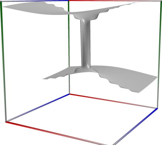

\(\quad\) \(\quad\)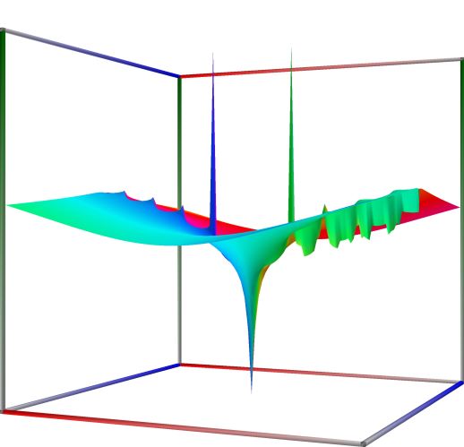

3D wpf plot: real part (left figure), imaginary part (middle figure) and absolute value with color-coded phase (right figure) of the complex sine function \(z = \sin(x + iy)\), with \(-6 \le x \le 6\) (blue axis), \(-6 \le y \le 6\) (red axis), \(-10 \le z \le 10\) (green axis). Function values are loglog-transformed.

An example in Python

>>> from xlcalcnet import ecplx
>>> ecplx.Rstheta(0.5)
ecplx('5.2359877559829887307E-1')
>>> ecplx.Rstheta('0.1')
ecplx('5.3518479027559984754E-1')

Hardy (or Riemann-Siegel) Z function

mathc53.hardy_z(z)

Returns the Hardy (or Riemann-Siegel) Z function. See also Wikipedia [1474], MathWorld [1092], NIST [14], Flint [833], Ehrhardt [309] (4.2.52), Mpmath [743].

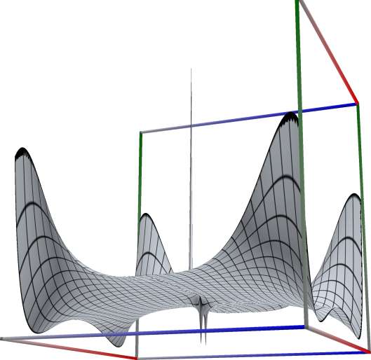
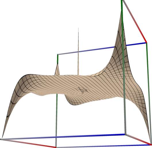
\[Z(t) = e^{i \theta(t)} \zeta(1/2+it)\]

where \(\zeta(s)\) is the Riemann zeta function and \(\theta(t)\) denotes the Riemann-Siegel theta function.

This calls acb_dirichlet_hardy_z.

Computes the Z-function, also known as the Riemann-Siegel Z function,

\[Z(t) = e^{i \theta(t)} \zeta(1/2+it)\]

where \(\zeta(s)\) is the Riemann zeta function (zeta()) and where \(\theta(t)\) denotes the Riemann-Siegel theta function (see siegeltheta()).

\(\quad\) \(\quad\)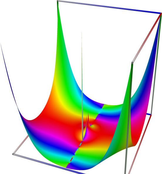

3D wpf plot: real part (left figure), imaginary part (middle figure) and absolute value with color-coded phase (right figure) of the complex sine function \(z = \sin(x + iy)\), with \(-6 \le x \le 6\) (blue axis), \(-6 \le y \le 6\) (red axis), \(-10 \le z \le 10\) (green axis). Function values are loglog-transformed.

An example in Python

>>> from xlcalcnet import ecplx
>>> ecplx.SiegelZ(0.5)
ecplx('5.2359877559829887307E-1')
>>> ecplx.SiegelZ('0.1')
ecplx('5.3518479027559984754E-1')

An example with real input:

>>> from xlcalcnet import dec, mpm, gmp, fpm, apm
>>> mpm.dps = 40; x = '2.6'
>>> \mathrm{d}x = dec.siegelz(x); mx = mpm.siegelz(x); gx = gmp.siegelz(x)
>>> fx = fpm.siegelz(x); ax = apm.siegelz(x)
>>> mpm.show([\mathrm{d}x, mx, gx, fx, ax])
dec:  -5.270127547934236224731698070416108808706E-1
mpm:  -5.270127547934236224731698070416108808706e-1
gmp:  -5.270127547934236224731698070416108808706E-01
fpm:  -5.27012754793424E-01
apm:  -5.270127547934236224731698070416108808706e-1 (-1.002e-37%)

An example with complex input:

>>> from xlcalcnet import dec, mpm, gmp, fpm, apm
>>> mpm.dps = 20; z = '2.6 + 3j'
>>> \mathrm{d}z = dec.siegelz(z); mz = mpm.siegelz(z); gz = gmp.siegelz(z)
>>> fz = fpm.siegelz(z); az = apm.siegelz(z)
>>> mpm.show([\mathrm{d}z, mz, gz, fz, az],  aligned=True)
dec: -2.8270067277806269605E-1               - 1.6028967412508714310E-1j
mpm: -2.8270067277806269605e-1               - 1.6028967412508714310e-1j
gmp: -2.8270067277806269605E-01              - 1.6028967412508714310E-01j
fpm: -2.82700672778063E-01                   - 1.60289674125087E-01j
apm: -2.8270067277806269605e-1 (-2.097e-18%) - 1.6028967412508714310e-1 (-4.228e-18%)j

Riemann (Landau) function \(\xi(s)\)

ctxflint.riemann_xi(s)

Returns the Riemann (Landau) function \(\xi(s)\). See also MathWorld [1089], Wikipedia [1461], Flint [828].

Landau’s lower-case \(\xi\) (“xi”) is defined as

\[\xi (s)={\frac {1}{2}}s(s-1)\pi ^{-s/2}\Gamma \left({\frac {s}{2}}\right)\zeta (s)\]

for \(s\in \mathbb {C}\). Here \(\zeta (s)\) denotes the Riemann zeta function and \(\Gamma (s)\) is the Gamma function. The functional equation (or reflection formula) for Landau’s \(\xi\) is

\[\xi (1-s)=\xi (s)\]

An example with real input:

>>> from xlcalcnet import dec, mpm, gmp, fpm, apm
>>> mpm.dps = 40; x = '2.6'
>>> \mathrm{d}x = dec.riemann_xi(x); mx = mpm.riemann_xi(x); gx = gmp.riemann_xi(x)
>>> fx = fpm.riemann_xi(x); ax = apm.riemann_xi(x)
>>> mpm.show([\mathrm{d}x, mx, gx, fx, ax])
dec:  5.502477451681679934572096474654698087218E-1
mpm:  5.502477451681679934572096474654698087218e-1
gmp:  5.502477451681679934572096474654698087218E-01
fpm:  5.50247745168168E-01
apm:  5.502477451681679934572096474654698087218e-1 (1.46e-38%)

An example with complex input:

>>> from xlcalcnet import dec, mpm, gmp, fpm, apm
>>> mpm.dps = 20; z = '2.6 + 3j'
>>> \mathrm{d}z = dec.riemann_xi(z); mz = mpm.riemann_xi(z); gz = gmp.riemann_xi(z)
>>> fz = fpm.riemann_xi(z); az = apm.riemann_xi(z)
>>> mpm.show([\mathrm{d}z, mz, gz, fz, az],  aligned=True)
dec: 4.2915713107054790438E-1              + 1.2956749025413144593E-1j
mpm: 4.2915713107054790438e-1              + 1.2956749025413144593e-1j
gmp: 4.2915713107054790438E-01             + 1.2956749025413144593E-01j
fpm: 4.29157131070548E-01                  + 1.29567490254131E-01j
apm: 4.2915713107054790437e-1 (1.974e-18%) + 1.2956749025413144593e-1 (6.537e-18%)j

Dirichlet eta function, \(\eta(s)\)

math53.dirichlet_eta(x)

Returns the Dirichlet eta function, defined as \(\displaystyle \eta(s) = (1 - 2^{1-s})\zeta(s) = \sum_{k=0}^{\infty} \frac{(-1)^k}{k^s}\) for \(s>0\) and by analytic continuation for \(s \le 0\).

See also: MathWorld [1071], Ehrhardt [309] (3.6.3.1), Flint [828], Mpmath [735].

An example in Python

>>> from xlcalcnet import ereal
>>> ereal.DirichletEta(12)
ereal('5.2359877559829887307E-1')
>>> ereal.DirichletEta('10.0001')
ereal('5.3518479027559984754E-1')

An example with real input:

>>> from xlcalcnet import dec, mpm, gmp, fpm, apm
>>> mpm.dps = 40; x = '2.6'
>>> \mathrm{d}x = dec.dirichlet_eta(x); mx = mpm.dirichlet_eta(x); gx = gmp.dirichlet_eta(x)
>>> fx = fpm.dirichlet_eta(x); ax = apm.dirichlet_eta(x)
>>> mpm.show([\mathrm{d}x, mx, gx, fx, ax])
dec:  8.748307349702805779574670518491745461882E-1
mpm:  8.748307349702805779574670518491745461882e-1
gmp:  8.748307349702805779574670518491745461882E-01
fpm:  8.74830734970281E-01
apm:  8.748307349702805779574670518491745461882e-1 (1.968e-39%)

An example with complex input:

>>> from xlcalcnet import dec, mpm, gmp, fpm, apm
>>> mpm.dps = 20; z = '2.6 + 3j'
>>> \mathrm{d}z = dec.dirichlet_eta(z); mz = mpm.dirichlet_eta(z); gz = gmp.dirichlet_eta(z)
>>> fz = fpm.dirichlet_eta(z); az = apm.dirichlet_eta(z)
>>> mpm.show([\mathrm{d}z, mz, gz, fz, az],  aligned=True)
dec: 1.0368930023009351181E+0              + 1.3961421241509646940E-1j
mpm: 1.0368930023009351181e+0              + 1.3961421241509646940e-1j
gmp: 1.0368930023009351181E+00             + 1.3961421241509646940E-01j
fpm: 1.03689300230094E+00                  + 1.39614212415096E-01j
apm: 1.0368930023009351181e+0 (1.634e-19%) + 1.3961421241509646940e-1 (6.825e-19%)j

Dirichlet \(\eta(s) - 1\)

math53.dirichlet_eta_m1(s)

Returns the Dirichlet function \(\eta(s)-1 = (\zeta(s)-1) - (2^{1-s} \zeta(s))\).

See also: MathWorld [1071], Ehrhardt [309] (3.6.3.3).

An example in Python

>>> from xlcalcnet import ereal
>>> ereal.DirichletEtam1(5)
ereal('5.2359877559829887307E-1')
>>> ereal.DirichletEtam1('51')
ereal('5.3518479027559984754E-1')

An example with real input:

>>> from xlcalcnet import dec, mpm, gmp, fpm, apm
>>> mpm.dps = 40; x = '2.6'
>>> \mathrm{d}x = dec.etam1(x); mx = mpm.etam1(x); gx = gmp.etam1(x)
>>> fx = fpm.etam1(x); ax = apm.etam1(x)
>>> mpm.show([\mathrm{d}x, mx, gx, fx, ax])
dec:  -1.251692650297194220425329481508254538118E-1
mpm:  -1.251692650297194220425329481508254538118e-1
gmp:  -1.251692650297194220425329481508254538118E-01
fpm:  -1.25169265029719E-01
apm:  -1.251692650297194220425329481508254538118e-1 (-1.376e-38%)

An example with complex input:

>>> from xlcalcnet import dec, mpm, gmp, fpm, apm
>>> mpm.dps = 20; z = '2.6 + 3j'
>>> \mathrm{d}z = dec.etam1(z); mz = mpm.etam1(z); gz = gmp.etam1(z)
>>> fz = fpm.etam1(z); az = apm.etam1(z)
>>> mpm.show([\mathrm{d}z, mz, gz, fz, az],  aligned=True)
dec: 3.6893002300935118091E-2              + 1.3961421241509646940E-1j
mpm: 3.6893002300935118091e-2              + 1.3961421241509646940e-1j
gmp: 3.6893002300935118091E-02             + 1.3961421241509646940E-01j
fpm: 3.68930023009351E-02                  + 1.39614212415096E-01j
apm: 3.6893002300935118089e-2 (4.592e-18%) + 1.3961421241509646940e-1 (6.825e-19%)j

Dirichlet beta function, \(\beta(s)\)

math53.dirichlet_beta(s)

Returns the Dirichlet beta function, defined as \(\displaystyle \beta(s) = \sum_{n=0}^{\infty} \frac{(-1)^n}{(2n+1)^s}\), for \(s>0\), and by analytic continuation for \(s \le 0\).

See also: Wikipedia [1448], MathWorld [1049], Ehrhardt [309] (3.6.4).

Alternatively, the following definition, in terms of the Hurwitz zeta function, is valid in the whole complex s-plane:

\[\beta (s)=4^{-s}\left(\zeta \left(s,{1 \over 4}\right)-\zeta \left(s,{3 \over 4}\right)\right).\]

An example in Python

>>> from xlcalcnet import ereal
>>> ereal.DirichletBeta(5)
ereal('5.2359877559829887307E-1')
>>> ereal.DirichletBeta('51')
ereal('5.3518479027559984754E-1')

An example with real input:

>>> from xlcalcnet import dec, mpm, gmp, fpm, apm
>>> mpm.dps = 40; x = '2.6'
>>> \mathrm{d}x = dec.dirichlet_beta(x); mx = mpm.dirichlet_beta(x); gx = gmp.dirichlet_beta(x)
>>> fx = fpm.dirichlet_beta(x); ax = apm.dirichlet_beta(x)
>>> mpm.show([\mathrm{d}x, mx, gx, fx, ax])
dec:  9.535048662378325267539346079940401993601E-1
mpm:  9.535048662378325267539346079940401993601e-1
gmp:  9.535048662378325267539346079940401993601E-01
fpm:  9.53504866237832E-01
apm:  9.535048662378325267539346079940401993601e-1 (1.084e-38%)

An example with complex input:

>>> from xlcalcnet import dec, mpm, gmp, fpm, apm
>>> mpm.dps = 20; z = '2.6 + 3j'
>>> \mathrm{d}z = dec.dirichlet_beta(z); mz = mpm.dirichlet_beta(z); gz = gmp.dirichlet_beta(z)
>>> fz = fpm.dirichlet_beta(z); az = apm.dirichlet_beta(z)
>>> mpm.show([\mathrm{d}z, mz, gz, fz, az],  aligned=True)
dec: 1.0550279685803642739E+0              + 3.3718823063670455627E-3j
mpm: 1.0550279685803642739e+0              + 3.3718823063670455627e-3j
gmp: 1.0550279685803642739E+00             + 3.3718823063670455627E-03j
fpm: 1.05502796858036E+00                  + 3.37188230636704E-03j
apm: 1.0550279685803642739e+0 (7.226e-19%) + 3.3718823063670455625e-3 (1.828e-16%)j

Dirichlet lambda function, \(\lambda(s)\)

math53.dirichlet_lambda(s)

Returns the Dirichlet lambda function, defined as \(\displaystyle \lambda(s) = \sum_{n=0}^{\infty} (2n+1)^{-s}, for `s>1\), and by analytic continuation for \(s < 1\).

See also: MathWorld [1073], Ehrhardt [309] (3.6.5), Hu and Kim [394].

The function is calculated as

\[\lambda(s) = (1-2^{-s}) \zeta(s) = -\text{exp2m1}(-s) \zeta(s)\]

An example in Python

>>> from xlcalcnet import ereal
>>> ereal.DirichletLambda(5)
ereal('5.2359877559829887307E-1')
>>> ereal.DirichletLambda('51')
ereal('5.3518479027559984754E-1')

An example with real input:

>>> from xlcalcnet import dec, mpm, gmp, fpm, apm
>>> mpm.dps = 40; x = '2.6'
>>> \mathrm{d}x = dec.dirichlet_lambda(x); mx = mpm.dirichlet_lambda(x); gx = gmp.dirichlet_lambda(x)
>>> fx = fpm.dirichlet_lambda(x); ax = apm.dirichlet_lambda(x)
>>> mpm.show([\mathrm{d}x, mx, gx, fx, ax])
dec:  1.090154272021530585919018418830832116026E+0
mpm:  1.090154272021530585919018418830832116026e+0
gmp:  1.090154272021530585919018418830832116026E+00
fpm:  1.09015427202153E+00
apm:  1.090154272021530585919018418830832116056e+0 (2.815e-36%)

An example with complex input:

>>> from xlcalcnet import dec, mpm, gmp, fpm, apm
>>> mpm.dps = 20; z = '2.6 + 3j'
>>> \mathrm{d}z = dec.dirichlet_lambda(z); mz = mpm.dirichlet_lambda(z); gz = gmp.dirichlet_lambda(z)
>>> fz = fpm.dirichlet_lambda(z); az = apm.dirichlet_lambda(z)
>>> mpm.show([\mathrm{d}z, mz, gz, fz, az],  aligned=True)
dec: 9.5326918762855854694E-1              + 2.2012809770791952023E-2j
mpm: 9.5326918762855854694e-1              + 2.2012809770791952023e-2j
gmp: 9.5326918762855854694E-01             + 2.2012809770791952023E-02j
fpm: 9.53269187628559E-01                  + 2.20128097707919E-02j
apm: 9.5326918762855854695e-1 (7.108e-19%) + 2.2012809770791952017e-2 (1.972e-17%)j

Zeros of the Riemann zeta function

ctxflint.zeta_zero(n)

Returns the zeros of the Riemann zeta function. See also Wikipedia [1473], MathWorld [1090], NIST [15], Mpmath [749].

This calls acb_dirichlet_zeta_zero.

Computes the \(n\)-th nontrivial zero of \(\zeta(s)\) on the critical line, i.e. returns an approximation of the \(n\)-th largest complex number \(s = \frac{1}{2} + ti\) for which \(\zeta(s) = 0\). Equivalently, the imaginary part \(t\) is a zero of the Z-function (siegelz()).

An example :

>>> from xlcalcnet import dec, mpm, gmp, fpm, apm
>>> mpm.dps = 20; n = '20'
>>> \mathrm{d}z = dec.zetazero(n); mz = mpm.zetazero(n); gz = gmp.zetazero(n)
>>> fz = fpm.zetazero(n); az = apm.zetazero(n)
>>> mpm.show([\mathrm{d}z, mz, gz, fz, az],  aligned=True)
dec: 5.0000000000000000000E-1        + 7.7144840068874805373E+1j
mpm: 5.0000000000000000000e-1        + 7.7144840068874805373e+1j
gmp: 5.0000000000000000000E-01       + 7.7144840068874805373E+01j
fpm: 5.00000000000000E-01            + 7.71448400688748E+01j
apm: 5.0000000000000000000e-1 (0.0%) + 7.7144840068874805373e+1 (7.027e-20%)j