Setting up XlCalcNet

Installing XlCalcNet

Installing a version of Python which is dedicated to MS Excel and/or LibreOffice Calc

The XlCalcNet package is compatible with Python versions 3.8 - 3.15. It is recommended to use a version of CPython which is both mature and supported. In this manual, we will use Python version 3.13.15.

Important

However, if we want to use XlCalcNet with LibreOffice (version 7.0 or later, 64 bit), we need to make sure that the version which we install is compatible with the main Python core installation of LibreOffice, which means that the first 2 numbers of the version number x.y.z must match.

To find out which version this is, follow these steps: In the folder C:\Program Files\LibreOffice\program double-click on python.exe. This opens the python console, which in the first line states which Python version is used. At the time of writing (October 2026), the most current version of LibreOffice is version 26.8, which uses Python version 3.13.15. Earlier version of LibreOffice use different versions of Python.

Python can be installed in different ways. It is recommended to install Python as a dedicated version for use with MS Excel and/or LibreOffice Calc, which does not require uninstalling any previous versions of Python, does not interfere with other Python installations, and does not require administrative privileges.

As installation folder any folder can be used for which the user has read and write access. In the following we will assume that the installation folder is C:\Python313. We assume that the path to this folder is NOT added to the PATH environment variable.

As an example of the installation process, we download the windows installer of version 3.13.15 (64 bit) from https://www.python.org/downloads/release/python-31315/. We will install this version into the folder C:\Temp, so we make sure beforehand that this folder exists and is empty.

In the Download folder, double-click on the downloaded file python-3.13.15-amd64.exe to start the installation. Click on “Customize installation”.

In the next dialog page “Optional Features” unselect “Documentation”, “Python test suite”, “py launcher” and “for all users”. Click on “Next”.

In the next dialog page “Advanced Options” unselect all items, including “Create shortcuts”. In the line below “Customize install location” enter C:\Temp. Click on Install. Once the installation has been completed, the last dialog page “Setup was successful” appears. Click on Close.

In the Windows explorer, navigate to the folder C:\Temp. Open another Windows explorer instance, navigate to C:\, and create the folder C:\Python313. Copy (DO NOT move!) the content of C:\Temp into C:\Python313.

Click the Start button and open Settings (or press Windows Key + I). Click on Apps on the left menu. Select Installed apps to view and manage all programs installed on your PC. Navigate to “Python 3.13.15 (64-bit)” and click on the ... symbol. Select Uninstall and confirm. Once Uninstall has been completed, the last dialog page “Uninstall was successful” appears. Click on Close.

Now the folder C:\Temp can be deleted. The folder C:\Python313 contains the (“freestanding”) Python version that we will work with in this manual.

First steps with XlCalcNet

Since the path to C:\Python313 is not added to the PATH environment variable, it is convenient to prepare, within the C:\Python313 folder, batch files for the installation of the Python packages which one wishes to install and possibly update later.

The first batch file will ensure that our version of pip is up to date. Right-click over any free space in the C:\Python313 folder, select New -> Text Document. Rename this document to A01upgradepip.bat, ignoring the warning. Open this file for editing in the Windows standard editor. Type python -m pip install -U --no-warn-script-location pip as install command, begin a new line, type pause, save the file, and close the editor.

Now double-click on A01upgradepip.bat. This will update pip as needed.

In the same way prepare a batch file named A02installxlcalcnet.bat, using python -m pip install -U  xlcalcnet as install command. Double-click on A02installxlcalcnet.bat. This will install the latest version of the XlCalcNet package.

To check that this installation was successful, double-click on python.exe, which will open the python console:

>>> from xlcalcnet import mpm
>>> mpm.dps = 40
>>> mpm.sqrt(2)
    mpf('1.414213562373095048801688724209698078569662')

The 3 folders which are used by XlCalcNet

XlCalcNet uses the following 3 folders:

• The installation folder (in our example C:\Python313\Lib\site-packages\xlcalcnet), which contains the program code of the package (which should not be changed by the user during normal use). This folder is automatically created during the installation of XlCalcNet.

• The DataXlCalcNet folder in the Documents folder, which contains code examples and data which are directly manipulated by the user. This folder needs to created manually by the user (see below).

• The XlCalcNetIDE folder in the AppDataLocal folder, which contains data or executable binaries which are generated as a result of running a Python script or C# program. This folder is automatically created while using XlCalcNet.

Important

It is crucial for the correct functioning of XlCalcNetThat that the DataXlCalcNet folder is located in the Documents folder. The DataXlCalcNet folder has already been downloaded during the installation of XlCalcNet; it is located in the installation folder (in our example C:\Python313\Lib\site-packages\xlcalcnet). The user needs to copy it manually from the installation folder into the Documents folder.

Preparing the use of additional installation batch files for installing Python packages

The DataXlCalcNet folder contains a number of batch files for installing additional Python packages which can be used with XlCalcNet. These batch files are located in the subfolder \PythonBatchFiles\BatchFiles. The user can copy these batch files into the C:\Python313 folder, and double-click on them to install the corresponding Python packages. The user can also create new batch files for installing additional Python packages, using the same procedure as described above for creating the batch files A01upgradepip.bat and A02installxlcalcnet.bat.

Installing and using Python.NET: Calling C# from Python

Python.NET is a package that gives Python programmers nearly seamless integration with the .NET Common Language Runtime (CLR) and provides a powerful application scripting tool for .NET developers. It allows Python code to interact with the CLR, and may also be used to embed Python into a .NET application.

See pythonnet/pythonnet

Assuming that the Python batch files have been installed as described here, Python.NET can be installed by double-clicking on the batch file A03installpythonnet.bat in the C:\Python313 folder.

To check that this installation was successful, double-click on python.exe, which will open the python console. With Python.NET installed, we can access the C# module qreal, which provides functions in quadruple precision:

>>> from xlcalcnet import qreal
>>> qreal.sqrt(2)
    qreal('1.4142135623730950488016887242097')

Soem background information:

.NET Framework is part of the Microsoft Windows operating system since Windows Vista; .NET Framework 4.x can be installed since Windows XP. Recent versions of Windows (Windows 7 - Windows 11), which have been kept fully maintained, have .NET Framework 4.8 installed, which is the latest version of .NET Framework and will continue to be distributed with future releases of Windows. As long as it is installed on a supported version of Windows, .NET Framework 4.8 will continue to also be supported (see https://dotnet.microsoft.com/en-us/platform/support/policy/dotnet-framework).

As part of the .NET Framework 4.x runtime, 3 different compilers are provided: csc.exe (C#), vbc.exe (Visual Basic), and jsc.exe (JScript).

The 32 bit targeting versions are located in C:\Windows\Microsoft.NET\Framework\v4.0.30319 and those for 64 bit in C:\Windows\Microsoft.NET\Framework64\v4.0.30319.

It is important to note that these compilers are not part of Visual Studio but part of Windows; they are, in a way, the closest to a compiler as part of the operating system that Windows has ever come up with. On the other hand, these compilers have been tugged away with the rest of the .NET Framework 4.x runtime; in that sense, they are “hidden” compilers.

In the following, we will ignore the Visual Basic and JScript compilers, but focus only on C#. The C# compiler supports only language versions up to C# 5. Luckily, this still provides us with all language features which we need for our purposes.

In terms of usability, the .NET Framework 4.x runtime does not include an IDE; we therefore include a Tiny IDE as described below.

Installing and using the Tiny IDE as a Python application

Installation

With the DataXlCalcNet folder in the Documents folder and Python.NET installed, we can start using the “Tiny C#/Python IDE”, which makes it easy to edit and run small programs written in Python or C#. The Tiny IDE is a Python program (it is started with pythonw.exe) which loads a UserControl written in C#. This is made possible by Python.NET.

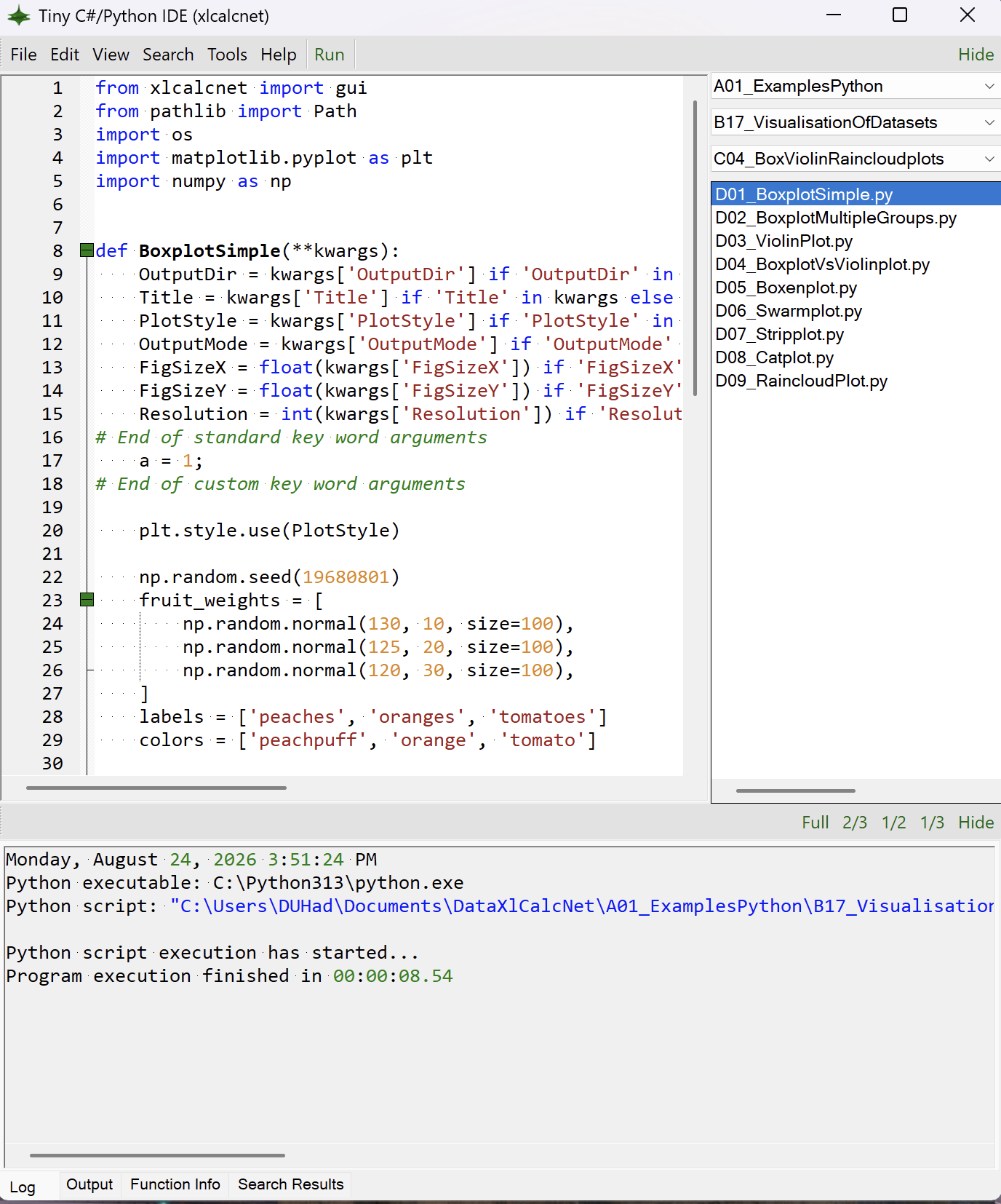
Follow these steps to make the Tiny IDE available:

• In the Python installation folder, rightclick on pythonw.exe.

• Select Create shortcut -> Result: pythonw.exe-Shortcut. (On Windows 11: Select Show more options -> Create shortcut -> Result: pythonw.exe-Shortcut.)

• Rightclick on pythonw.exe-shortcut; Select Properties.

• In the dialogue Properties, select “Target”, and type:C:\Python313\pythonw.exe C:\Users\DUHad\Documents\DataXlCalcNet\A01_ExamplesPython\B01_GeneralUsage\C01_Setup\D03_ShowEditor.py. Here the path to the documents folder (in our case C:\Users\DUHad\Documents) needs to be changed to meet the settings of your system. Then save.

• Rename pythonw.exe-Shortcut to TinyIDE_Python313

• Doubleclick on TinyIDE_Python313

• In the task-bar, right-click on the appearing Python symbol, and select “Pin to taskbar”

From now on, you can start the Tiny IDE by clicking on this Python symbol on the taskbar. To start an additional instance of the Tiny IDE when the Tiny IDE is already running, click in the main menu on Tools -> Tiny IDE (external). Note that the Python source code for starting the Tiny IDE is also the Python code example which is shown after starting the Tiny IDE (in A01_ExamplesPython\B01_GeneralUsage\C01_Setup\D03_ShowEditor.py), so clicking on Run will also start an additional instance. However, now the program does not return until it is closed, as it is not running in an additional instance of Python; running the program like this is useful for debugging and testing purposes, like modifying title, width and height of the window, which can be changed on lines 67-68.

Overview

The Tiny IDE is designed around the structure of the DataXlCalcNet folder, making it easy to navigate and manage existing code examples, as well a new code written by the user. The Tiny IDE can be used only to edit and run Python or C# code examples which are located in the DataXlCalcNet folder and are located in subfolders beginning with A0. The code examples are organized in a tree structure, which is shown in the top right panel (the “folder panel”) of the Tiny IDE.

The top left panel (the “editor panel”) of the Tiny IDE shows the code of the selected file, which can be edited and run. The Tiny IDE also provides features like syntax highlighting, autocompletion, bookmarks, code folding, and error highlighting to make coding easier.

The output of the program is shown in the bottom panel (the “output panel”) of the Tiny IDE, which has 4 tabs: the “Log” tab, which documents the progress of compiling and running the code (and also displays warning and error messages); the “Output” tab, which shows the text output of the program (if any); the “Function Info” tab, which provides information about the functions (if they belong to a module from XlCalcNet); and the “Search Results” tab, which shows the search results.

Each file in the DataXlCalcNet\A0* folders can be opened in the Tiny IDE by clicking on it. Per Tiny IDE instance, only one file can be opened, edited and run at a time (to open an additional file, you need to start a new instance of the Tiny IDE: Tools -> Tiny IDE (external)). The Tiny IDE will load this file into the editor, and the code can be edited and run. To run the code, click on the “Run” button in the main menu. The output of the program (if any) is shown in the output tab of the output panel.

The ordering and naming of the code examples in the subfolders A01_ExamplesPython and A02_ExamplesCSharp matches the ordering and naming of the corresponding chapters, sections and subsections in this manual, making it easy to find the code example which corresponds to a specific section of the manual. In addition, the “section help” feature (Help -> Section Help), which is available in the main menu of the Tiny IDE and opens the corresponding section of this manual in a web browser, depends on this ordering and naming.

Also, in Python, the feature that code examples can be called like modules, using statements like from A01_ExamplesPython.B17_VisualisationOfDatasets.C01_BarCharts import D01_BarChartPart1, depends on keeping this ordering and naming intact.

Therefore the names of these folders and files should not be changed, and new code examples should be added to the appropriate folders, either A03_UserlibPython or A04_UserlibCSharp for user-defined libraries, or A05_UserExamplesPython or A06_UserExamplesCSharp for code examples which demonstrate the use of existing or user-defined libraries. The Tiny IDE will automatically detect new files and folders, and will update the tree structure accordingly.

The menu bar of the Editor

The Menubar of the Tiny IDE contains the following menus: File, Edit, View, Search, Tools, and Help. Each menu contains a number of items, which are described below.

There are also two buttons (with green foreground color) in the menu bar: the “Run” button, which runs the code of the current file, and the “Show/Hide” button, which toggles the visibility of the folder panel.

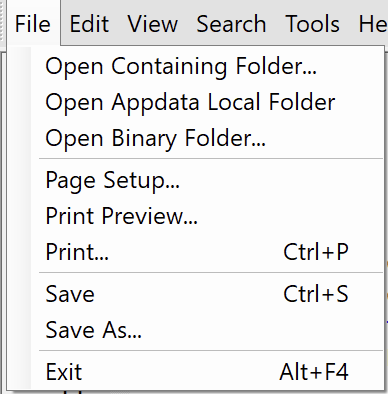
In the File menu, two standard items are missing: “New” and “Open”.

The “New” item is missing because the Tiny IDE is designed to work within the DataXlCalcNet folder, and therefore new files which are not in the current folder should be created in the appropriate subfolders of DataXlCalcNet, which often have to be created manually first using the Windows Explorer.

There is, however, a Save As item in the file menu, which allows to save the current file under a new name in the current folder. This is useful for creating a copy of an existing file, and using this as a starting point for a new file.

The “Open” item (which would typically open a dialog box with the functionally of the Windows Explorer) is missing because the Tiny IDE is limited to the DataXlCalcNet folder. Instead the folder panel allows to navigate through the DataXlCalcNet folder and open any file in it.

Renaming or deleting files and folders is possible, but should be done with care, using the Windows Explorer, and not using the Tiny IDE. After these changes, when returning to the Tiny IDE, the tree structure will not be updated automatically, but has to be updated manually by clicking on the appropriate parent folder in the tree structure.

Open Containing Folder opens the Windows Explorer in the folder of the current file. This is useful for quickly accessing other files in the same folder, or for deleting files and folders.

Open Appdata Local Folder opens the Windows Explorer in the AppData\Local\XlCalcNetIDE folder. This is useful for quickly accessing files and folders which are generated by running Python or C# code examples in the Tiny IDE.

Open Binary Folder opens the Windows Explorer in the Bin subfolder of the XlCalcNet installation. This is useful mostly for debugging purposes.

Page Setup opens the standard Windows dialog for setting up the page layout for printing. Print Preview opens a preview of the current file, which can be printed from there. Print opens the standard Windows dialog for printing the current file.

Save will just save the current file without any further action. Save As has been descibed above. Exit will close the Tiny IDE.

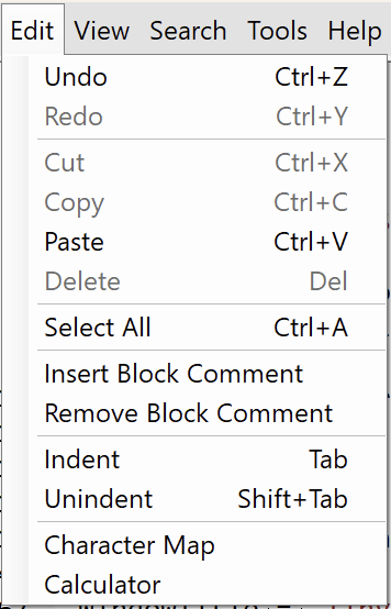
In the Edit menu, Undo, Redo, Cut, Copy, Paste, Delete, and Select All are standard items. Insert BlockComment and Remove BlockComment allows to comment or uncomment a block of code, which is useful for testing purposes (these 2 items are available in the context menu as well). Indent and Unindent allow to indent or unindent a block of code, which is useful for formatting purposes.

Character Map opens the standard Windows dialog for selecting special characters, which can be inserted into the code. Calculator opens the standard Windows calculator, which can be used for quick calculations.

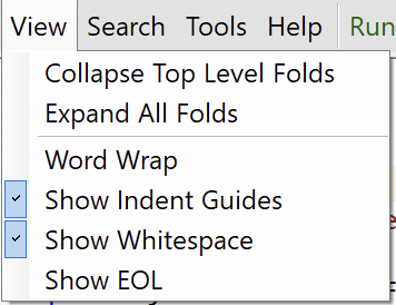
In the View menu, Collapse Top Level Folds allows to collapse all top level folds in the code, which is useful for quickly navigating through the code.

Expand All Folds allow to collapse or expand all folds in the code, which will make all code visible

Show Indentation Guides toggles the visibility of indentation guides in the editor panel.

Word Wrap toggles word wrap in the editor panel.

Show Whitespace toggles the visibility of whitespace characters in the editor panel.

Show EOL toggles the visibility of end of line markers in the editor panel.

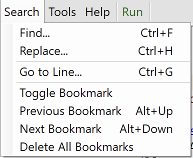
In the Search menu, Find starts the search for a string in the code, Replace allows to replace a string in the code, and Goto allows to jump to a specific line number in the code.

The corresponding dialog boxes are shown below:

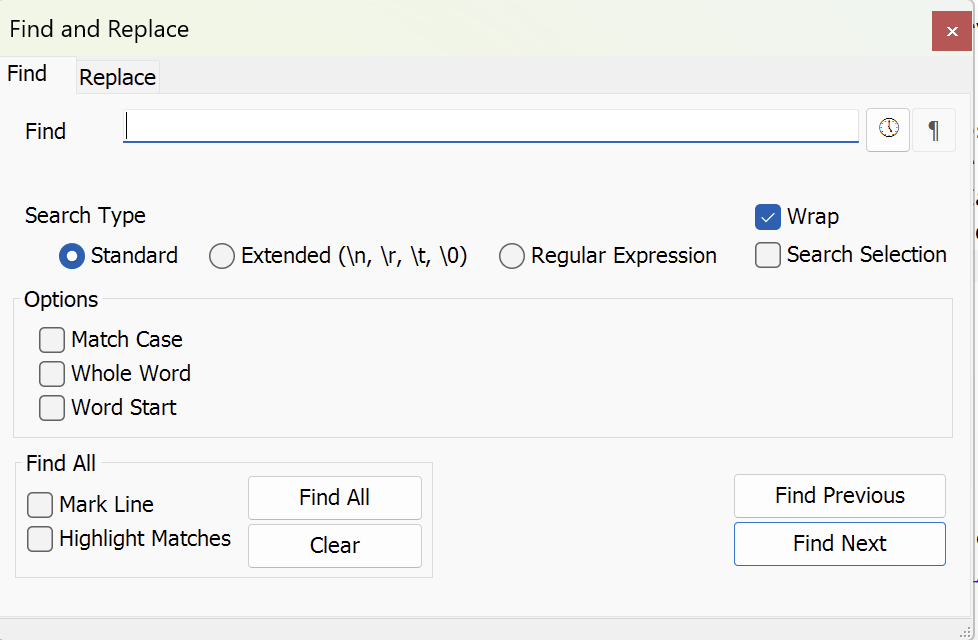
If the string is found, the first occurrence is highlighted in the code. If the string is not found, a message box appears which informs that the string was not found. The search can be continued by clicking on Find Next or Find Previous. The search can be limited to the current selection, and it can be case sensitive or insensitive. The search can also be done using regular expressions.

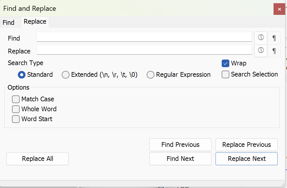
If the string is found, the first occurrence is highlighted in the code. If the string is not found, a message box appears which informs that the string was not found. The search can be continued by clicking on Find Next or Find Previous. Replace Next, Replace Previous or Replace All can be used to decide what to do with the found string. The search can be limited to the current selection, and it can be case sensitive or insensitive. The search can also be done using regular expressions.

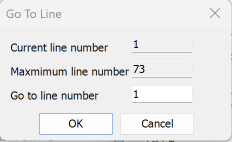
if the line number is valid, the cursor jumps to the specified line number. If the line number is invalid, a message box appears which informs that the line number is invalid.

Toggle Bookmark allows to set or delete a bookmark in the code, which can be used to quickly navigate through the code. Delete All Bookmarks deletes all bookmarks in the code. Next Bookmark jumps to the next bookmark in the code. Previous Bookmark jumps to the previous bookmark in the code.

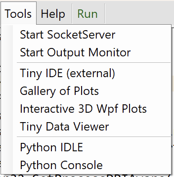
In the Tools menu, Start Socket Server starts the socket server, see here for details.

Start Output Monitor starts the output monitor application, see here for details.

Tiny IDE (external) starts an additional instance of the Tiny IDE, which can be used to edit and run another file.

Gallery of Plots starts the gallery of plots application, see here for details.

Interactive 3D Wpf Plots starts the Interactive 3D Wpf Plots application, see here for details.

Tiny Data Viewer starts the Tiny Data Viewer application, see here for details.

Python IDLE starts the Python IDLE application.

Python Console starts the Python console.

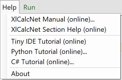
In the Help menu, XlCalcNet Manual (online)... displays the start page of the XlCalcNet online manual in a web browser.

XlCalcNet Section Help (online)... displays the section of the XlCalcNet.online manual which corresponds to the current file in a web browser.

Tiny IDE Tutorial (online)... displays the section of the XlCalcNet.online manual which explains the use of the Tiny IDE in a web browser.

Python Tutorial (online)... displays the online tutorial for Python, which is available on the official Python website in a web browser.

C\# Tutorial (online)... displays the online tutorial for C#, which is available on the official C# website in a web browser.

About XlCalcNet... displays information about the XlCalcNet package, including version number and copyright information.

The context menu of the editor

Right-clicking in the editor panel opens a context menu, which provides quick access to common actions like Insert Block, Remove Block Comment, Collapse Top Level Folds, Expand All Folds, Goto Previous Bookmark, Goto Next Bookmark, all of which are also available in the main menu.

New in this context menu is the item Show Function Info, which for functions which belong to a module from XlCalcNet, displays information about the function in the “Function Info” tab of the output panel.

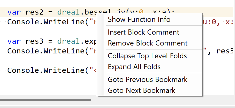
In the screenshot above, the context menu is shown after right-clicking on the function dreal.bessel_jv (with the curser to the right of the dot). The item Show Function Info is highlighted, and the corresponding information about this function is shown in the “Function Info” tab of the output panel below.

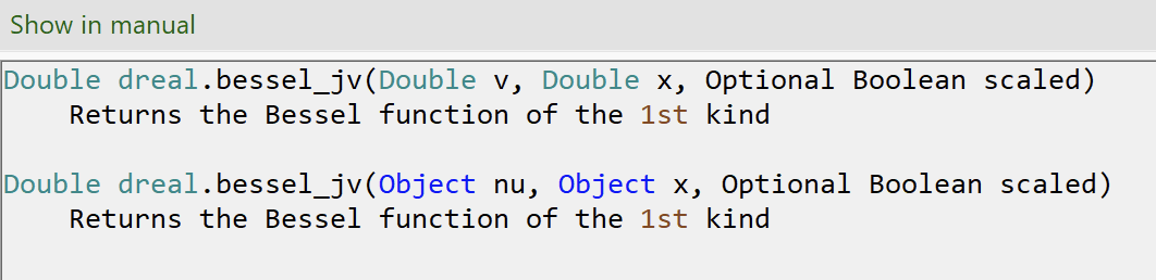
Just to the upper left of the Show Function Info item, the button Show in Manual is visible. Clicking on this button opens the corresponding section of the XlCalcNet online manual in a web browser.

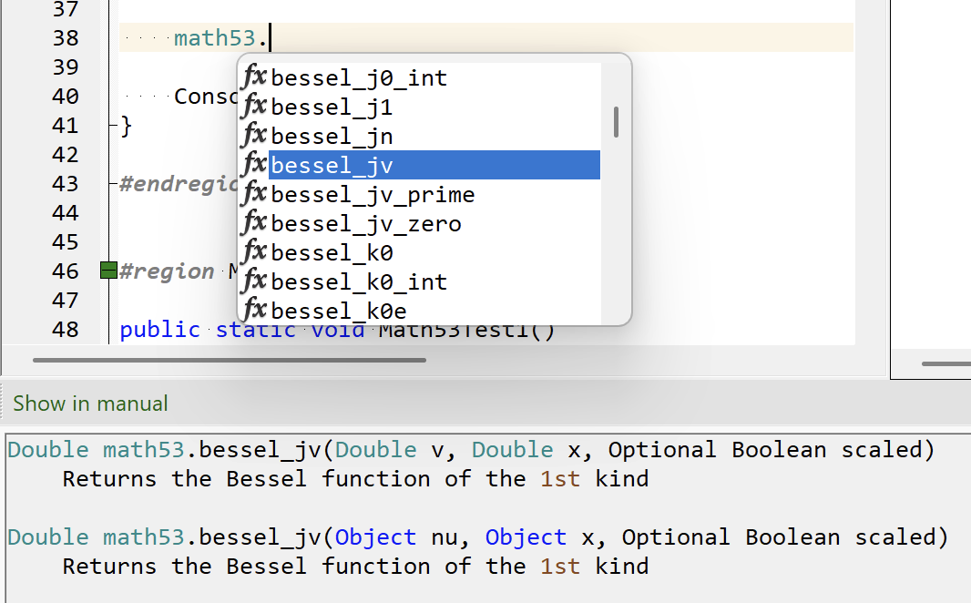
This works in combination with the autocomplete feature, which is activated by pressing Ctrl + Space. The autocomplete feature shows a list of functions which belong to a module from XlCalcNet, and for each function, the corresponding information is shown in the “Function Info” tab of the output panel. This allows to quickly find the function which is needed, and to see how it can be used.

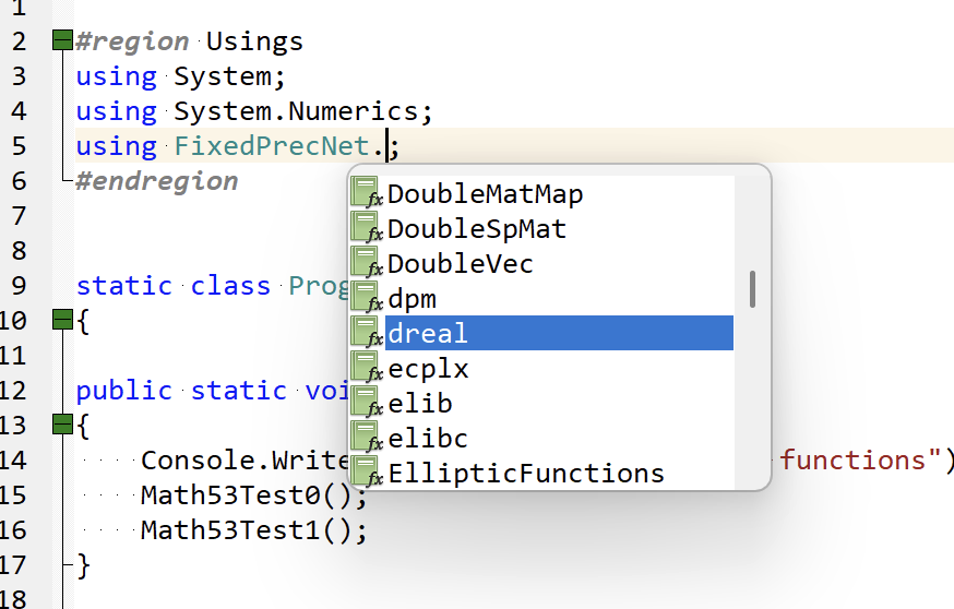
The autocomplete feature also works for user-defined libraries, however in these cases no additional information is shown in the “Function Info” tab of the output panel.

The Python development cycle in the Tiny IDE

Here we describe the Python development cycle in the Tiny IDE for producing and running python programs. The process for producing a Python library is similar but different, and is described here.

Overall, the Python development cycle in the Tiny IDE consists of the following steps: The file is opened in the editor panel, and the code is edited as needed. The code can be run by clicking on the “Run” button in the main menu bar. If there are any errors or warnings, they are shown in the “Log” tab of the output panel. When clicking on the error messages in the “Log” tab, they are also highlighted in the code. After correcting the errors, the “Run” button can be clicked again. If there are no errors, the code is is executed. Any text output of the program is shown in the “Output” tab of the output panel after the program has finished running.

These steps are illustrated in the following screenshots, which show the Python development cycle in the Tiny IDE for producing and running python programs.

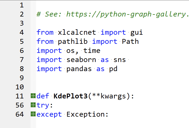
Directly after loading the Python code example, the code is folded, and the “Log” tab of the output panel is empty. The “Output” tab of the output panel is also empty, since the program has not been run yet. The unfolded code looks like this:

# See: https://python-graph-gallery.com/80-contour-plot-with-seaborn/

from xlcalcnet import gui
from pathlib import Path
import os, time
import seaborn as sns
import pandas as pd

def KdePlot3(**kwargs):
    OutputDir = kwargs['OutputDir'] if 'OutputDir' in kwargs else 'OutputMonitor'
    Title = kwargs['Title'] if 'Title' in kwargs else 'KdePlot3'
    PlotStyle = kwargs['PlotStyle'] if 'PlotStyle' in kwargs else 'default'
    OutputMode = kwargs['OutputMode'] if 'OutputMode' in kwargs else 'svg'
    FigSizeX = float(kwargs['FigSizeX']) if 'FigSizeX' in kwargs else 4
    FigSizeY = float(kwargs['FigSizeY']) if 'FigSizeY' in kwargs else 4
    Resolution = int(kwargs['Resolution']) if 'Resolution' in kwargs else 300
# End of standard key word arguments

    # Choose 'Agg' as backend unless we want to display the graphics
    if (OutputMode != 'gui'):
        import matplotlib
        matplotlib.use('Agg')
    import matplotlib.pyplot as plt
    plt.style.use(PlotStyle)

    fn = gui.get_dataxlcalcnet()
    fn += r'\DataExamples\MainExamples\Workbooks\Datasets.xlsx'
    datasets = pd.ExcelFile(fn)
    df = pd.read_excel(datasets, 'iris')

    sns.set_style('white')
    sns.kdeplot(x=df.sepal_width, y=df.sepal_length,
                cmap='Blues', fill=True, bw_adjust=0.5)

    fig = plt.gcf()
    fig.tight_layout()


# Start of output choices
    if (OutputMode == 'plt'):
        plt.show()
    elif (OutputMode == 'gui'):
        gui.plot(fig, __file__, Title)
    else:
        FName = 'Temp'
        if OutputDir != 'Temp': FName = (Path(__file__).stem)
        LocalDir = gui.get_local_appdata_xlcalcnet()
        FullPath = os.sep.join([LocalDir, OutputDir, FName + '.' + OutputMode])
        plt.savefig(FullPath,  bbox_inches='tight')
        if OutputDir != 'Temp': print('Graphics written to: ', FullPath)
    plt.close('all')

try:
    if __name__ == '__main__':
        start0 = time.time()
        KdePlot3(OutputMode = 'gui')
        end0 = time.time()
        print('Elapsed time:', format(end0 - start0, '.4g'), 'seconds' )


except Exception:
    import traceback
    print(traceback.format_exc())

Folding in Python works on code blocks which are defined by indentation. At the top of the file are the import statements, followed by a def funcname(**kwargs) statement, where “funcname” in this case is KdePlot3. The body of this function is the place where “the real work” is done.

This function also has two standardized parts (for Matplotlib graphic code examples), one at the beginning, which takes care of the keyword arguments and ensures that the ‘Agg’ backend is used unless one wants to display the graphics (this is necessary to ensure this function can be called from older versions of Libreoffice like 7.4); and another at the end (”# Start of output choices”), which makes sure that interactive use, output to the OutputMonitor folder, or output to another folder is possible in verious formats (like jpg, png, svg, pdf).

At the end of the file, the try ... except block makes sure that exceptions are dealt with properly, that the time for actually running the code (as opposed to the time required to load and initialize the imported libraries) is printed, and that we have the chance to call the function with a specific set of keyword arguments (in this case OutputMode = 'gui').

Python files with this overall structure are well suited for calls from within spreadsheet functions.

The output of the program is shown in the “Output” tab of the output panel after the program has finished running. Lengthy text output can be folded and unfolded, and the context menu allows to copy the output to the clipboard, clear the output, or save the output to a file.

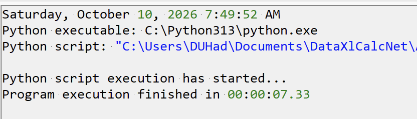
The “Log” tab of the output panel contains additional information after successfully running the program.

The snapshot above shows a code snippet which contains an error (print is misspelled as print2``)

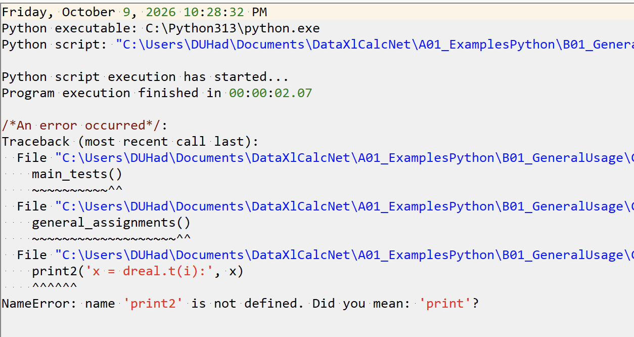
This error is detected by the Python interpreter, and is reported in the Log tab of the output panel.

After double-clicking in the Log tab on the first line in red color, the error is also indicated in the editor, with a full error message below the line where the error occured.

The CSharp development cycle in the Tiny IDE

Here we describe the C# development cycle in the Tiny IDE for producing *.exe files which are stored in the AppData\Local\XlCalcNetIDE\Bin folder, and which can be run immediately. The process for producing *.dll files which can be called from Python is similar but different, and is described here.

Overall, the C# development cycle in the Tiny IDE consists of the following steps: The file is opened in the editor panel, and the code is edited as needed. The code can be compiled by clicking on the “Run” button in the main menu bar. If there are any errors or warnings, they are shown in the “Log” tab of the output panel. When clicking on the error messages in the “Log” tab, they are also highlighted in the code. After correcting the errors, the “Run” button can be clicked again to compile the code. If there are no errors, the code is compiled into a *.exe file, which is stored in the AppData\Local\XlCalcNetIDE\Bin folder and which is executed automatically after successful compilation. Any text output of the program is shown in the “Output” tab of the output panel after the program has finished running.

These steps are illustrated in the following screenshots, which show the C# development cycle in the Tiny IDE for producing *.exe files:

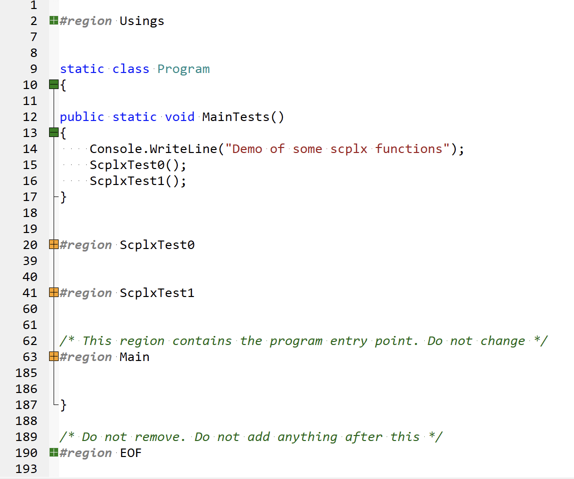
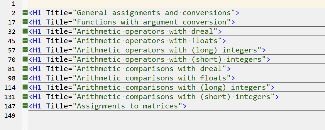
Directly after loading the C# code example, the code is folded, and the “Log” tab of the output panel is empty. The “Output” tab of the output panel is also empty, since the program has not been run yet.

Folding in C# works both on regions and on code blocks. Overall, the folding of regions is more important than the folding of code blocks, since it allows to hide the implementation of functions and classes, and to focus on the overall structure of the code. The folding of code blocks is useful for hiding the implementation of loops and conditional statements, and to focus on the overall structure of the code.

The screenshot above shows the overall structure of the C# code examples in XlCalcNet, which are organized into regions. The first region contains the using statements, followed (outside of any region) by a static class Program statement, and the first function in this class, which always has the form public static void MainTests(). The body of this function contains calls to the functions where “the real work” is done.

The implementations of these functions are located in the following regions (in this example the regions “ScplxTest0” and “ScplxTest1”), which are organized according to the functionality of the functions. The next region is called “Main”, and contains the implementation of the Main function, which is the entry point of the program, and contains a lot of necessary boilerplate code, which makes sure that the program can run without a project file (which Visual Studio would require). The last region is called “EOF”, and makes sure that code folding is working properly (adressing a small bug in the underlying ScintillaNet library). These last two regions should never be changed by the user during normal use.

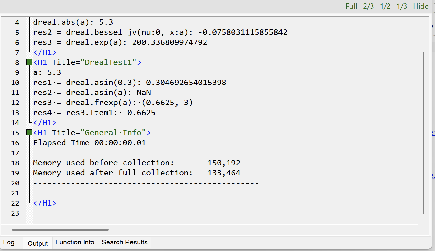
The output of the program is shown in the “Output” tab of the output panel after the program has finished running. The output can be folded and unfolded, and the context menu allows to copy the output to the clipboard, clear the output, or save the output to a file.

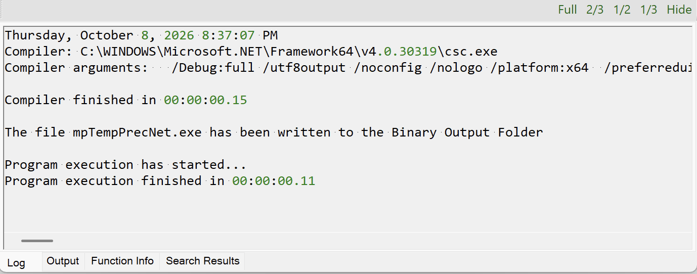
The “Log” tab of the output panel contains additional information after successfully compiling and running the program.

The snapshot above shows a code snippet which contains an error (the variable res1 is defined twice)

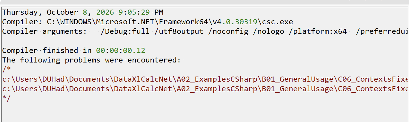
This error is detected by the compiler, and is reported in the Log tab of the output panel.

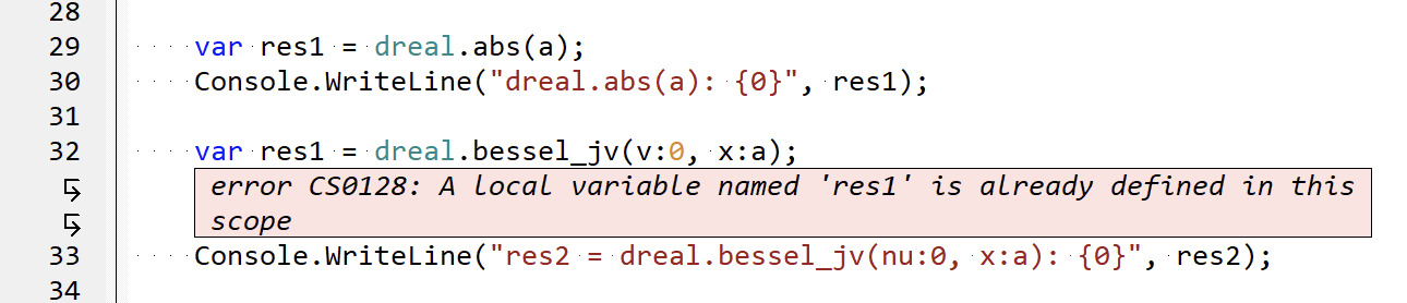
After double-clicking in the Log tab on the first line in red color, the error is also indicated in the editor, with a full error message below the line where the error occured.

Warnings are treated in a way similar to errors: in this case the program is compiled (in the absence of errors), but is not run. Instead the warning is shown in the Log tab, and after double-clicking on it the warning is also indicated in the editor, with a full error message below the line where the warning was triggered.

The Output tab in the Output Panel

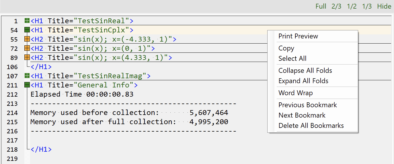
Describe the toolbar on top of the Output tab.

Note that the Output tab in the Output Panel can be used to display any text output of a Python or C# program. The output can be folded and unfolded, and the context menu allows to copy the output to the clipboard, clear the output, or save the output to a file.

Source code

The Python source code for starting the IDE can be found here: duhadler/XlCalcNet

The C# source code for the IDE can be found here: duhadler/XlCalcNet

Installing and using Numpy, Matplotlib, Pandas, Scipy, Seaborn, Statsmodels and Scikit-learn

Numpy

Numpy is “The fundamental package for scientific computing with Python”. For more information, see https://numpy.org/ and https://en.wikipedia.org/wiki/NumPy.

Assuming that the Python batch files have been installed as described here, Numpy can be installed by double-clicking on the batch file A04installnumpy.bat in the C:\Python313 folder.

The following example shows how Numpy can be used with the Decimal type to calculate the mean:

import numpy as np
from xlcalcnet import dpm

def demo_mp():
    r = 8
    c = 2
    dpm.dps = 30
    R = np.ndarray((r,c),dtype=dpm.realtype)
    d1 = dpm.t(1.0)
    for i in range(r):
        for j in range(c):
            R[i,j] = 10*(i+1) + d1/(j+7)
    print(R)
    print()
    res = np.mean(R)
    print("res = np.mean(R): \n", res, type(res))
    print()
    res = np.mean(R, axis=0)
    print("res = np.mean(R, axis=0): \n", res, type(res))
    print()
    res = np.mean(R, axis=1)
    print("res = np.mean(R, axis=1): \n", res, type(res))

def demo_all():
    demo_mp()

demo_all()

The output looks like this:

[[Decimal('10.1428571428571428571428571429') Decimal('10.125')]
 [Decimal('20.1428571428571428571428571429') Decimal('20.125')]
 [Decimal('30.1428571428571428571428571429') Decimal('30.125')]
 [Decimal('40.1428571428571428571428571429') Decimal('40.125')]
 [Decimal('50.1428571428571428571428571429') Decimal('50.125')]
 [Decimal('60.1428571428571428571428571429') Decimal('60.125')]
 [Decimal('70.1428571428571428571428571429') Decimal('70.125')]
 [Decimal('80.1428571428571428571428571429') Decimal('80.125')]]

res = np.mean(R):
 45.1339285714285714285714285715 <class 'decimal.Decimal'>

res = np.mean(R, axis=0):
 [Decimal('45.142857142857142857142857143') Decimal('45.125')] <class 'numpy.ndarray'>

res = np.mean(R, axis=1):
 [Decimal('10.1339285714285714285714285714')
 Decimal('20.1339285714285714285714285714')
 Decimal('30.1339285714285714285714285714')
 Decimal('40.1339285714285714285714285714')
 Decimal('50.1339285714285714285714285715')
 Decimal('60.1339285714285714285714285715')
 Decimal('70.1339285714285714285714285715')
 Decimal('80.1339285714285714285714285715')] <class 'numpy.ndarray'>

Matplotlib

Matplotlib is “a comprehensive library for creating static, animated, and interactive visualizations in Python”. For more information, see https://matplotlib.org/ and https://en.wikipedia.org/wiki/Matplotlib.

Assuming that the Python batch files have been installed as described here, Matplotlib can be installed by double-clicking on the batch file A05installmatplotlib.bat in the C:\Python313 folder.

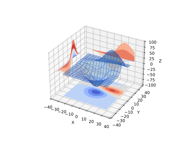
The following example shows how Matplotlib can be used to produce a boxplot. This code example shows how parameters can be passed:

The Python code for the example below can also be found online in the DataXlCalcNet repository or in the corresponding local DataXlCalcNet folder in the file D04b_Matplotlib3D.py.

from xlcalcnet import gui
import os, re
import numpy as np
import mpl_toolkits.mplot3d.axes3d as axes3d
import matplotlib.pyplot as plt

def ProjectFilledContour(**kwargs):
    OutputDir = kwargs['OutputDir'] if 'OutputDir' in kwargs else 'OutputMonitor'
    Title = kwargs['Title'] if 'Title' in kwargs else 'ProjectFilledContour'
    PlotStyle = kwargs['PlotStyle'] if 'PlotStyle' in kwargs else 'default'
    OutputMode = kwargs['OutputMode'] if 'OutputMode' in kwargs else 'gui'
    FigSizeX = float(kwargs['FigSizeX']) if 'FigSizeX' in kwargs else 4
    FigSizeY = float(kwargs['FigSizeY']) if 'FigSizeY' in kwargs else 4
    Resolution = int(kwargs['Resolution']) if 'Resolution' in kwargs else 300
# End of standard key word arguments

    plt.style.use(PlotStyle)

    fig = plt.figure()
    ax = fig.add_subplot(projection='3d')
    X, Y, Z = axes3d.get_test_data(0.05)

    # Plot the 3D surface
    ax.plot_surface(X, Y, Z, edgecolor='royalblue', lw=0.5, rstride=8, cstride=8,
                    alpha=0.3)

    # Plot projections of the contours for each dimension.  By choosing offsets
    # that match the appropriate axes limits, the projected contours will sit on
    # the 'walls' of the graph
    ax.contourf(X, Y, Z, zdir='z', offset=-100, cmap='coolwarm')
    ax.contourf(X, Y, Z, zdir='x', offset=-40, cmap='coolwarm')
    ax.contourf(X, Y, Z, zdir='y', offset=40, cmap='coolwarm')

    ax.set(xlim=(-40, 40), ylim=(-40, 40), zlim=(-100, 100),
           xlabel='X', ylabel='Y', zlabel='Z')
    fig.tight_layout()

# Start of output choices
    if (OutputMode == 'gui'):
        gui.plot(fig, __file__, Title)
    else:
        FName = 'Temp'
        if OutputDir != 'Temp': FName = re.sub('[^a-zA-Z0-9]', '', Title)
        LocalDir = gui.get_local_appdata_xlcalcnet()
        FullPath = os.sep.join([LocalDir, OutputDir, FName])
        plt.savefig(FullPath + '.' + OutputMode,  bbox_inches='tight')
    plt.close('all')

try:
    if __name__ == '__main__':
        ProjectFilledContour()

except Exception:
    import traceback
    print(traceback.format_exc())

This produces the following output:

Pandas

Pandas is “a fast, powerful, flexible and easy to use open source data analysis and manipulation tool, built on top of the Python programming language”. For more information, see https://pandas.pydata.org/ and https://en.wikipedia.org/wiki/Pandas_(software)

Assuming that the Python batch files have been installed as described here, Pandas can be installed by double-clicking on the batch file A06installpandas.bat in the C:\Python313 folder.

The following example shows how Pandas can be used to access data in an Excel workbook:

import time
import pandas as pd

def main_tests():
    get_irisdata()

def get_documents_folder():
    """Returns the documents folder."""
    import ctypes, ctypes.wintypes
    buf = ctypes.create_unicode_buffer(ctypes.wintypes.MAX_PATH)
    ctypes.windll.shell32.SHGetFolderPathW(None, 0x0005, None, 0, buf)
    return str(buf.value)

def get_irisdata():
    fn = get_documents_folder()
    fn += r'\DataXlCalcNet\DataExamples\MainExamples\Workbooks\Datasets.xlsx'
    datasets = pd.ExcelFile(fn)
    df = pd.read_excel(datasets, 'iris')
    print(df)
    print(df.head(8))
    print(df.dtypes)

try:
    if __name__ == '__main__':
        start0 = time.time()
        main_tests()
        end0 = time.time()
        print('Elapsed time:', format(end0 - start0, '.4g'), 'seconds' )

except Exception:
    import traceback
    print(traceback.format_exc())

The output looks like this:

     Sepal.Length  Sepal.Width  Petal.Length  Petal.Width    Species
0             5.1          3.5           1.4          0.2     setosa
1             4.9          3.0           1.4          0.2     setosa
2             4.7          3.2           1.3          0.2     setosa
3             4.6          3.1           1.5          0.2     setosa
4             5.0          3.6           1.4          0.2     setosa
..            ...          ...           ...          ...        ...
145           6.7          3.0           5.2          2.3  virginica
146           6.3          2.5           5.0          1.9  virginica
147           6.5          3.0           5.2          2.0  virginica
148           6.2          3.4           5.4          2.3  virginica
149           5.9          3.0           5.1          1.8  virginica

[150 rows x 5 columns]
   Sepal.Length  Sepal.Width  Petal.Length  Petal.Width Species
0           5.1          3.5           1.4          0.2  setosa
1           4.9          3.0           1.4          0.2  setosa
2           4.7          3.2           1.3          0.2  setosa
3           4.6          3.1           1.5          0.2  setosa
4           5.0          3.6           1.4          0.2  setosa
5           5.4          3.9           1.7          0.4  setosa
6           4.6          3.4           1.4          0.3  setosa
7           5.0          3.4           1.5          0.2  setosa
Sepal.Length    float64
Sepal.Width     float64
Petal.Length    float64
Petal.Width     float64
Species          object
dtype: object
Elapsed time: 0.4529 seconds

Scipy

Scipy is “a fast, powerful, flexible and easy to use open source data analysis and manipulation tool, built on top of the Python programming language”. For more information, see https://scipy.org/ and https://en.wikipedia.org/wiki/SciPy.

Assuming that the Python batch files have been installed as described here, Scipy can be installed by double-clicking on the batch file A07installscipy.bat in the C:\Python313 folder.

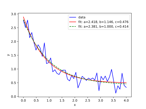
The following example shows how Scipy can be used for fitting data:

import numpy as np
import matplotlib.pyplot as plt
from scipy.optimize import curve_fit

def func(x, a, b, c):
    return a * np.exp(-b * x) + c

def test_curvefit():
    # See https://docs.scipy.org/doc/scipy/reference/generated/scipy.optimize.curve_fit.html
    print('Hello from test_curvefit!')

    xdata = np.linspace(0, 4, 50)
    y = func(xdata, 2.5, 1.3, 0.5)
    rng = np.random.default_rng()
    y_noise = 0.2 * rng.normal(size=xdata.size)
    ydata = y + y_noise
    plt.plot(xdata, ydata, 'b-', label='data')

    popt, pcov = curve_fit(func, xdata, ydata)
    print(popt)
    plt.plot(xdata, func(xdata, *popt), 'r-',
             label='fit: a=%5.3f, b=%5.3f, c=%5.3f' % tuple(popt))

    popt, pcov = curve_fit(func, xdata, ydata, bounds=(0, [3., 1., 0.5]))
    print(popt)
    plt.plot(xdata, func(xdata, *popt), 'g--',
             label='fit: a=%5.3f, b=%5.3f, c=%5.3f' % tuple(popt))

    plt.xlabel('x')
    plt.ylabel('y')
    plt.legend()
    plt.show()

try:
    print()
    test_curvefit()

except Exception:
    import traceback
    print(traceback.format_exc())

This produces the following output:

Seaborn

Seaborn is “a Python data visualization library based on matplotlib. It provides a high-level interface for drawing attractive and informative statistical graphics”. For more information, see https://seaborn.pydata.org/.

Assuming that the Python batch files have been installed as described here, Seaborn can be installed by double-clicking on the batch file A08installseaborn.bat in the C:\Python313 folder.

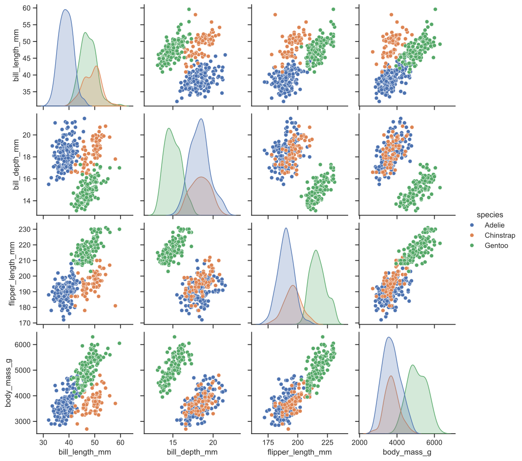
The following example shows how Seaborn can be used to produce a scatterplot matrix:

from xlcalcnet import gui
from pathlib import Path
import os
import seaborn as sns
import matplotlib.pyplot as plt

# See also: https://seaborn.pydata.org/examples/scatterplot_matrix.html

def ScatterplotMatrix(**kwargs):
    OutputDir = kwargs['OutputDir'] if 'OutputDir' in kwargs else 'OutputMonitor'
    Title = kwargs['Title'] if 'Title' in kwargs else 'ScatterplotMatrix'
    PlotStyle = kwargs['PlotStyle'] if 'PlotStyle' in kwargs else 'default'
    OutputMode = kwargs['OutputMode'] if 'OutputMode' in kwargs else 'svg'
    FigSizeX = float(kwargs['FigSizeX']) if 'FigSizeX' in kwargs else 4
    FigSizeY = float(kwargs['FigSizeY']) if 'FigSizeY' in kwargs else 4
    Resolution = int(kwargs['Resolution']) if 'Resolution' in kwargs else 300
# End of standard key word arguments

    plt.style.use(PlotStyle)

    sns.set_theme(style='ticks')
    df = sns.load_dataset('penguins')
    sns.pairplot(df, hue='species')
    fig = plt.gcf()

# Start of output choices
    if (OutputMode == 'plt'):
        plt.show()
    elif (OutputMode == 'gui'):
        gui.plot(fig, __file__, Title)
    else:
        FName = 'Temp'
        if OutputDir != 'Temp': FName = (Path(__file__).stem)
        LocalDir = gui.get_local_appdata_xlcalcnet()
        FullPath = os.sep.join([LocalDir, OutputDir, FName + '.' + OutputMode])
        plt.savefig(FullPath,  bbox_inches='tight')
        if OutputDir != 'Temp': print('Graphics written to: ', FullPath)
    plt.close('all')

try:
    if __name__ == '__main__':
        ScatterplotMatrix(OutputMode='gui')

except Exception:
    import traceback
    print(traceback.format_exc())

This produces the following output:

Statsmodels

Statsmodels is a Python package for statistical computations. For more information, see https://www.statsmodels.org/stable/index.html.

Assuming that the Python batch files have been installed as described here, Statsmodels can be installed by double-clicking on the batch file A09installstatsmodels.bat in the C:\Python313 folder.

The following example shows how Statsmodels can be used for ordinary least squares calculations:

import time
import numpy as np
import pandas as pd
import statsmodels.api as sm

# See also: https://www.statsmodels.org/stable/examples/notebooks/generated/ols.html


def OLS(**kwargs):

# End of standard key word arguments

    nsample = 100
    x = np.linspace(0, 10, 100)
    X = np.column_stack((x, x**2))
    beta = np.array([1, 0.1, 10])
    e = np.random.normal(size=nsample)

    X = sm.add_constant(X)
    y = np.dot(X, beta) + e

    model = sm.OLS(y, X)
    results = model.fit()
    print(results.summary())


try:
    if __name__ == '__main__':
        start0 = time.time()
        OLS()
        end0 = time.time()
        print('Elapsed time:', format(end0 - start0, '.4g'), 'seconds' )

except Exception:
    import traceback
    print(traceback.format_exc())

The output looks like this

                            OLS Regression Results
==============================================================================
Dep. Variable:                      y   R-squared:                       1.000
Model:                            OLS   Adj. R-squared:                  1.000
Method:                 Least Squares   F-statistic:                 4.027e+06
Date:                Sun, 11 Oct 2026   Prob (F-statistic):          2.61e-239
Time:                        08:43:02   Log-Likelihood:                -146.41
No. Observations:                 100   AIC:                             298.8
Df Residuals:                      97   BIC:                             306.6
Df Model:                           2
Covariance Type:            nonrobust
==============================================================================
                 coef    std err          t      P>|t|      [0.025      0.975]
------------------------------------------------------------------------------
const          1.6938      0.312      5.422      0.000       1.074       2.314
x1            -0.1856      0.144     -1.286      0.202      -0.472       0.101
x2            10.0215      0.014    717.320      0.000       9.994      10.049
==============================================================================
Omnibus:                        2.046   Durbin-Watson:                   2.207
Prob(Omnibus):                  0.359   Jarque-Bera (JB):                1.489
Skew:                          -0.065   Prob(JB):                        0.475
Kurtosis:                       2.416   Cond. No.                         144.
==============================================================================

Notes:
[1] Standard Errors assume that the covariance matrix of the errors is correctly specified.
Elapsed time: 0.005406 seconds

Scikit-learn

Scikit-learn is a Python package for machine learning. For more information, see https://scikit-learn.org/stable/index.html.

Assuming that the Python batch files have been installed as described here, Scikit-learn can be installed by double-clicking on the batch file A10install_scikit_learn.bat in the C:\Python313 folder.

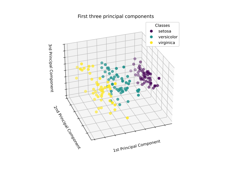
The following example shows how Scikit-learn can be used for a Principal Component Analysis (PCA) on the Iris dataset.:

from xlcalcnet import gui
from pathlib import Path
import os, time
import numpy as np
from sklearn.decomposition import PCA

# see https://scikit-learn.org/stable/auto_examples/decomposition/plot_pca_iris.html

def PlotPCA(**kwargs):
    OutputDir = kwargs['OutputDir'] if 'OutputDir' in kwargs else 'OutputMonitor'
    Title = kwargs['Title'] if 'Title' in kwargs else 'First three principal components'
    PlotStyle = kwargs['PlotStyle'] if 'PlotStyle' in kwargs else 'default'
    OutputMode = kwargs['OutputMode'] if 'OutputMode' in kwargs else 'svg'
    FigSizeX = float(kwargs['FigSizeX']) if 'FigSizeX' in kwargs else 8
    FigSizeY = float(kwargs['FigSizeY']) if 'FigSizeY' in kwargs else 6
    Resolution = int(kwargs['Resolution']) if 'Resolution' in kwargs else 300
# End of standard key word arguments

    # Choose 'Agg' as backend unless we want to display the graphics
    if (OutputMode != 'gui'):
        import matplotlib
        matplotlib.use('Agg')
    import matplotlib.pyplot as plt
    plt.style.use(PlotStyle)

    from sklearn.datasets import load_iris
    iris = load_iris(as_frame=True)
    #print(iris.keys())
    fig = plt.figure(1, figsize=(FigSizeX, FigSizeY))
    ax = fig.add_subplot(111, projection='3d', elev=-150, azim=110)

    X_reduced = PCA(n_components=3).fit_transform(iris.data)
    scatter = ax.scatter(
        X_reduced[:, 0],
        X_reduced[:, 1],
        X_reduced[:, 2],
        c=iris.target,
        s=40,
    )
    ax.set(
        title=Title,
        xlabel='1st Principal Component',
        ylabel='2nd Principal Component',
        zlabel='3rd Principal Component',
    )
    ax.xaxis.set_ticklabels([])
    ax.yaxis.set_ticklabels([])
    ax.zaxis.set_ticklabels([])

    # Add a legend
    legend1 = ax.legend(
        scatter.legend_elements()[0],
        iris.target_names.tolist(),
        loc='upper right',
        title='Classes',
    )
    ax.add_artist(legend1)

# Start of output choices
    if (OutputMode == 'plt'):
        plt.show()
    elif (OutputMode == 'gui'):
        gui.plot(fig, __file__, Title)
    else:
        FName = 'Temp'
        if OutputDir != 'Temp': FName = (Path(__file__).stem)
        LocalDir = gui.get_local_appdata_xlcalcnet()
        FullPath = os.sep.join([LocalDir, OutputDir, FName + '.' + OutputMode])
        plt.savefig(FullPath,  bbox_inches='tight')
        if OutputDir != 'Temp': print('Graphics written to: ', FullPath)
    plt.close('all')

try:
    if __name__ == '__main__':
        start0 = time.time()
        PlotPCA(OutputMode = 'gui')
        end0 = time.time()
        print('Elapsed time:', format(end0 - start0, '.4g'), 'seconds' )

except Exception:
    import traceback
    print(traceback.format_exc())

The output looks like this:

Calling Python from C:#: socket server vs in-process calls

A running socket server is critical for the use of XlCalcNet from Microsoft Excel.

When starting the socket server for the first time from a specific installation of python.exe, a dialog will appear to allow access of this version of Python to networks.

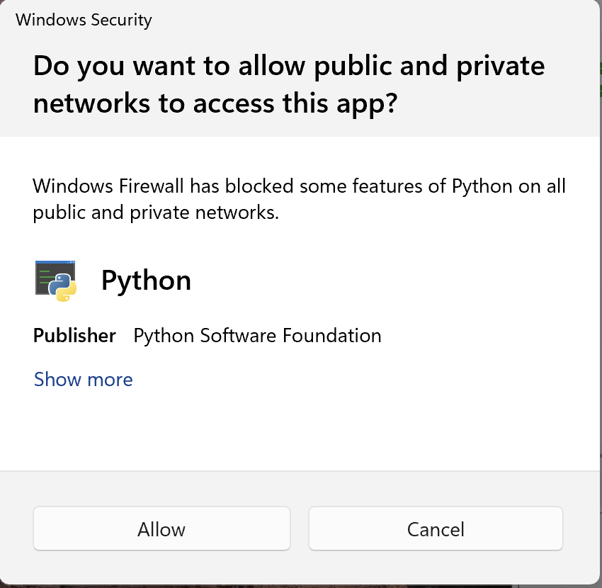
Confirm, since this is required for the socket server to work properly. If you have multiple installations of Python, you may have to do this for each installation.

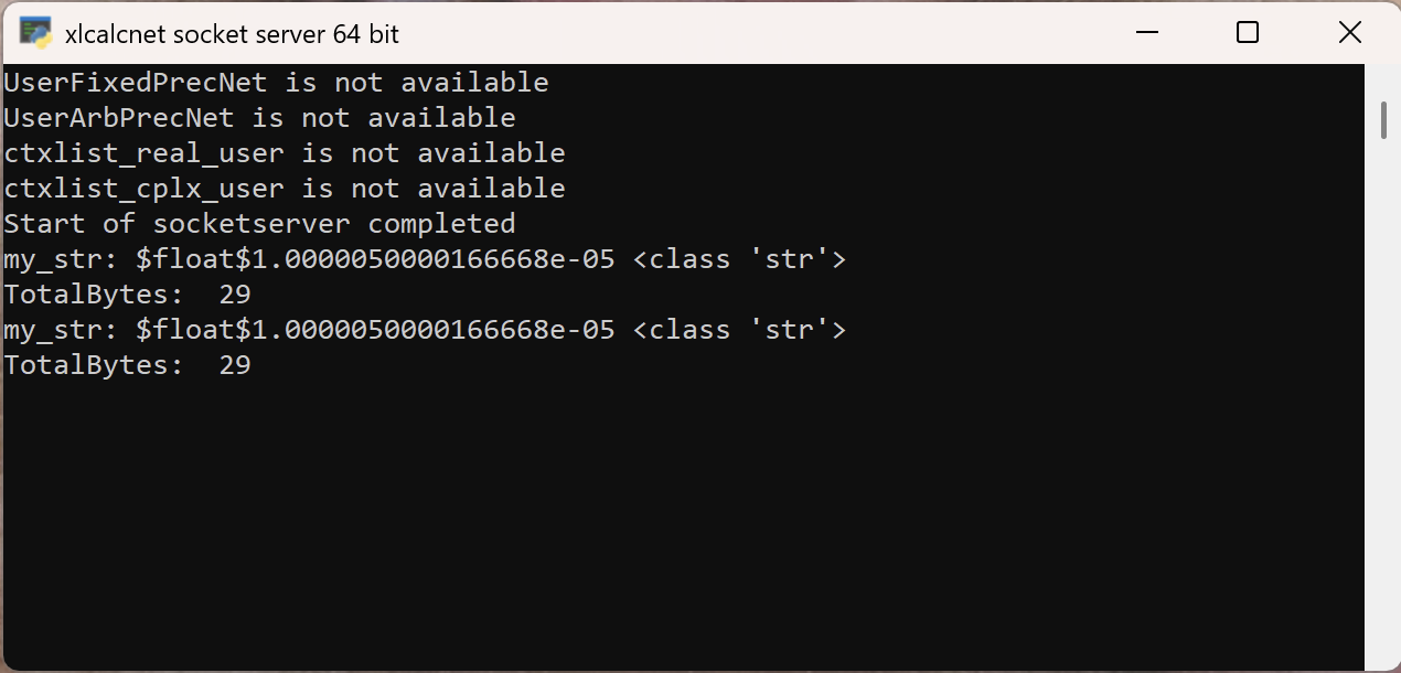
The socketserver is started from the TinyIDE: in the main menu, click on Tools -> Start SocketServer.

Calling the socketserver from C#

The full C# source code of the example below can be found online in the DataXlCalcNet repository or in the corresponding local DataXlCalcNet folder in the file D05a_CallSocketServer.cs.

The following example illustrates the use:

#region Usings
using MpFunLabClient;
using System;
using System.Diagnostics;
using System.Globalization;
using System.Threading;
using System.Numerics;
using FixedPrecNet;
#endregion

static class Program
{

public static void MainTests()
{
    Console.WriteLine("Demo of call socket server");
    for (int i = 0; i < 1; i++)
        TestSocketServer();
}

public static void TestSocketServer()
{
    Console.WriteLine("Hello TestSocketServer!");
    bool Transpose = false;
    bool ShowShape = true;

    string Code2 = "from A01_ExamplesPython.B18_FunctionsAndCurvesPlots.C02_BasicCurves import D02_Circle;";
    Code2 += "D02_Circle.CircleXY(); result = 'Done'";

    dynamic ResultFinal = MpFunLabSocketClientClass.CallSocketServer0(Code2, Transpose, ShowShape);
    Console.WriteLine();
    Console.WriteLine("Returned:");
    Console.WriteLine("{0}, {1}", ResultFinal.ToString(), ResultFinal.GetType());

    try
    {
        int U0 = ResultFinal.GetUpperBound(0);
        int U1 = ResultFinal.GetUpperBound(1);
        Console.WriteLine("U0: {0}, U1: {1}", U0, U1);
        for (int i = 0; i <= U0; i++)
        {
            for (int j = 0; j <= U1; j++)
            {
                Console.WriteLine("{0}, {1}", ResultFinal[i, j], ResultFinal[i, j].GetType());
            }
        }
    }
    catch (Exception)
    {
    }
    Console.WriteLine();
}

The Python source code for the socketserver itself can be found here: duhadler/XlCalcNet

The C# source code for the socket client which is called by the above program can be found here: duhadler/XlCalcNet

Calling Python from C# in-process

With Pythonnet, it is possible to call python from C# in-process. For the purposes of XlCalcNet this method is slower than calling the socket server. However, in other use cases, it might be the preferred method.

The full C# source code of the example below can be found online in the DataXlCalcNet repository or in the corresponding local DataXlCalcNet folder in the file D05b_TestPythonNet.cs.

The following example illustrates the use. Note that this requires including a using Python.Runtime; statement (line 6), passing the full path of the Python root directory(line 61), the Python DLL path (line 62) and setting a number of environment variables (lines 87-90). The Python engine must be initialized before any Python code can be executed (line 22):

#region Usings
using System;
using System.Collections.Generic;
using System.Numerics;
using FixedPrecNet;
using Python.Runtime;
#endregion

static class Program
{

public static void MainTests()
{
    TestPythonNet0();
}

#region TestPythonNet0

public static void TestPythonNet0()
{
    Console.WriteLine("Hello TestPythonNet1");
    PythonEngine.Initialize();
    using (Py.GIL())
    {
        dynamic np = Py.Import("numpy");
        Console.WriteLine(np.cos(np.pi * 2));

        dynamic sin = np.sin;
        Console.WriteLine(sin(5));

        double c = (double)(np.cos(5) + sin(5));
        Console.WriteLine(c);

        dynamic a = np.array(new List<float> { 1, 2, 3 });
        Console.WriteLine(a.dtype);

        dynamic b = np.array(new List<float> { 6, 5, 4 }, dtype: np.int32);
        Console.WriteLine(b.dtype);

        Console.WriteLine(a * b);
    }
}

#endregion



/* This region contains the program entry point. Do not change */
#region Main

public static void Main(string[] args)
{
    if (args.Length < 2)
    {
        Console.WriteLine(
            "This application needs to be started with 2 arguments;");
        Console.WriteLine("See the manual of xlcalcnet for details.");
    }
    else
    {
        _PythonRootDir = args[0];
        _PythonNetPyDll = args[1];
        _LocalAppDataDir = Environment.GetFolderPath(Environment.SpecialFolder
            .LocalApplicationData);
        AppDomain currentDomain = AppDomain.CurrentDomain;
        currentDomain.AssemblyResolve +=
            new ResolveEventHandler(LoadFromXlCalcNet);
        currentDomain.AssemblyResolve +=
            new ResolveEventHandler(LoadFromXlCalcNet2);
        currentDomain.AssemblyResolve +=
            new ResolveEventHandler(LoadFromPythonNet);
        currentDomain.AssemblyResolve +=
            new ResolveEventHandler(LoadFromAppLocal);
        System.Threading.Thread.CurrentThread.CurrentCulture =
            new System.Globalization.CultureInfo("en-US");
        System.Threading.Thread.CurrentThread.CurrentUICulture =
            new System.Globalization.CultureInfo("en-US");
        var ci = (System.Globalization.CultureInfo)System.Threading.Thread
            .CurrentThread.CurrentCulture.Clone();
        ci.NumberFormat.NegativeInfinitySymbol = "-Inf";
        ci.NumberFormat.PositiveInfinitySymbol = "+Inf";
        System.Threading.Thread.CurrentThread.CurrentCulture = ci;
        var stopWatch = new System.Diagnostics.Stopwatch();
        stopWatch.Start();
        try
        {
            Environment.SetEnvironmentVariable("PYTHONHOME", _PythonRootDir);
            Environment.SetEnvironmentVariable("PYTHONPATH", _PythonRootDir);
            Environment.SetEnvironmentVariable("PYTHONNET_PYDLL",
                _PythonNetPyDll);
            MainTests();
        }
        catch (Exception Ex)
        {
            Console.Error.WriteLine(Ex.Message);
            Console.Error.WriteLine("$+$");
            Console.Error.WriteLine(Ex.StackTrace);
            Console.Error.WriteLine("$+$");
        }
        stopWatch.Stop();
        var ts = stopWatch.Elapsed;
        string elapsedTime = string.Format("{0:00}:{1:00}:{2:00}.{3:00}",
            ts.Hours, ts.Minutes, ts.Seconds, ts.Milliseconds / 10);
        Console.WriteLine("<H1 Title=" + "\"" + "General Info" + "\"" + ">");
        Console.WriteLine("Elapsed Time " + elapsedTime);
        Console.WriteLine("------------------------------------------------");
        Console.WriteLine("Memory used before collection:       {0:N0}",
            GC.GetTotalMemory(false));
        GC.Collect();
        Console.WriteLine("Memory used after full collection:   {0:N0}",
            GC.GetTotalMemory(true));
        Console.WriteLine("------------------------------------------------");
        Console.WriteLine("");
        Console.WriteLine("</H1>");
    }

}

private static string _PythonRootDir;
private static string _PythonNetPyDll;
private static string _LocalAppDataDir;

/*
    The code for LoadFromXlCalcNet, LoadFromXlCalcNet2, LoadFromPythonNet
    and LoadFromAppLocal is not shown here
*/


#endregion


}

Running the program produces the following output:

Hello TestPythonNet1
1.0
-0.9589242746631385
-0.675262089199912
float64
int32
[ 6. 10. 12.]
<H1 Title="General Info">
Elapsed Time 00:00:00.58
------------------------------------------------
Memory used before collection:       5,854,328
Memory used after full collection:   1,431,368
------------------------------------------------

</H1>

In other words, it took about 0.58 seconds to run the program. This is much slower than calling the socket server, which takes about 0.02 seconds. The reason for this is that Pythonnet has to load the entire Python interpreter into the C# process, which takes a lot of time and memory. In contrast, the socket server runs in a separate process and can be started once and then used for multiple calls from C#.

Reasons for using multiprecision arithmetic

An introduction to the problems of rounding errors and catastrophic cancellation can be found in Goldberg [351]. Excellent reference texts are Higham [370] and Higham [371].

In the following sections we will give a few examples of how the use of double precision without special precaution can give wrong results.

Example: Sums

Sums are often calculated exactly if all summands have an exact representation. If this is not the case, results can be unpredictable. In MS Excel, the formula

=SUM(10000000000,-16000000000,6000000000)

will give the correct result \(0\), but the analogous formula

=SUM(1E+40,-1.6E+40,6E+39)

returns \(1.20893E+24\) instead of the correct result \(0\).

Example: Standard Deviation

Like sums, variances and standard deviations are often calculated exactly if all arguments have an exact representation. If this is not the case, results can again be unpredictable. In MS Excel, the formula

=VAR(1E+30,1E+30,1E+30)

returns \(2.97106E+28\) instead of the correct result \(0\), which should be the obvious results since all arguments are the same.

Example: Overflow and underflow

In many situations where the final result is representable in double precision, some of the interim results cause overflow or underflow. A popular example is the function \(f(x,y) = \sqrt{x^2+y^2}\). With \(x=3 \cdot 10^{300}\) and \(y=4 \cdot 10^{300}\) the result \(f(x,y) = 5 \cdot 10^{300}\) is representable in double precision, but the (naive) calculation will overflow.

Example: Polynomials

Consider the following example from Cuyt et al. [190]:

For \(a=77617\) and \(b=33096\), calculate

\[Y = 333.75 b^6 + a^2 (11 a^2 b^2 - b^6 - 121 b^4 - 2) + 5.5 b^8 + \frac{a}{2b}\]

The correct result is \(Y = -54767 / 66192 = -8.27396\ldots \cdot 10^{-1}\)

Example: Trigonometric Functions

Trigonometric functions are sensitive to small perturbations.

In double precision and binary floating point arithmetic, the tangent of \(x = 1.57079632679489\) is calculated as \(\tan(x) = 1.48752 \cdot 10^{14}\), whereas the correct result is \(\tan(x) = 1.51075 \cdot 10^{14}\). This amounts to an absolute error of \(2.32287 \cdot 10^{12}\) and a relative error of \(1.54\%\).

There are also limits on the range of arguments, e.g. \(\sin(10^{8})\) returns the value \(-9.31639 \cdot 10^{-1}\) (with an relative error of \(-6.22776 \cdot 10^{-13}\)), whereas \(\sin(10^{9})\) returns an invalid result (the exact result is \(5.45843 \cdot 10^{-1}\))

Example: Logarithms and Exponential Functions

Consider the following example from Kaveh R. Ghazi and Vincent Lefèvre and Philippe Théveny and Paul Zimmermann [1505]:

Determine 10 decimal digits of the constant

\[Y = 173746a + 94228b - 78487c, \quad \text{where }\]

\[a = \sin(10^{22}), b = \log(17.1), c = \exp(0.42).\]

The expected result is \(Y = -1.341818958 \cdot 10^{-12}\).

Example: Linear Algebra

The following example is from W. Hofschuster and W. Krämer [1506]:

We want to solve the (ill-conditioned) system of linear equations \(Ax = b\) with

\[\begin{split}A = \begin{pmatrix} a_{11} & a_{12} \\ a_{21} & a_{22} \end{pmatrix} = \begin{pmatrix} 64919121 & -159018721 \\ 41869520.5 & -102558961 \end{pmatrix}, b = \begin{pmatrix} b_{1} \\ b_{2} \end{pmatrix} = \begin{pmatrix} 1 \\ 0 \end{pmatrix} , x = \begin{pmatrix} x_{1} \\ x_{2} \end{pmatrix}\end{split}\]

The correct solution is \(x_1 = 205117922\), \(x_2 = 83739041\).

To solve this \(2 \times 2\) system numerically we first use the well known formulas

\[x_1 = \frac{a_{22}}{a_{11}a_{22} - a_{12}a_{21}}, \quad x_2 = \frac{-a_{21}}{a_{11}a_{22} - a_{12}a_{21}},\]

Calculating this directly in double precision gives the following wrong result:

\(x_1 = 102558961\), \(x_2 = 41869520.5\)

Example: Eigenvalues

The following example is from Brown et al. [161]:

The behaviour and stability of many physical systems are connected with the spectral properties of non-self-adjoint operators. However, numerical approximations of eigenvalues of non-selfadjoint operators (even matrices) may fail dramatically. For example, the non-normal 7 \(\times\) 7 matrix

\[\begin{split}A = \begin{pmatrix} 289 & 2054 & 326 & 128 & 70 & 32 & 6 \\ 1152 & 30 & 1312 & 512 & 288 & 128 & 32 \\ -29 & -1990 & 766 & 384 & 1018 & 224 & 58 \\ 512 & 128 & 640 & 0 & 640 & 512 & 128 \\ 1053 & 2246 & -514 & -384 & -766 & 800 & 198 \\ -287 & -6 & 1722 & -128 & 1978 & -30 & -2042 \\ -2176 & -285 & -1563 & -512 & -539 & -1152 & -287 \end{pmatrix}\end{split}\]

has the eigenvalues \(-2, -4, 0, 1, 1, 2, 4\). Calculations in double precision yield a set of complex eigenvalues, such as \(8.57 \pm 3.73 i; 2.29 \pm 8.33 i; -5.43 \pm 6.56 i; -8.85\) with imaginary parts as large as \(8.33\), which are nowhere near the true eigenvalues. The reason for this is that owing to the nonnormality of the matrix, its eigenvalues are highly sensitive to perturbations, and therefore unavoidable rounding errors render the numerical eigenvalue computations unreliable.

Rebuilding the .dll files of XlCalcNet and XlCalcNet2 from source code

The XlCalcNet and XlCalcNet2 python packages contain both precompiled .dll files and their source code.

This section descibes how to rebuild the .dll files of XlCalcNet and XlCalcNet2 from source code, either completely or only in part. The building process itself is not particularly difficult, but it requires the installation of MSYS2 (version 3.4.9.x86_64 or later: about 4 GB in size), Free Pascal (version 2.6.4 or later: about 320 MB in size), and Visual Studio Community (version 2019 or later: about 4.6 GB in size).

In the following it is assumed that the user has installed MSYS2, Free Pascal and Visual Studio Community and is comfortable using them.

MSYS2 is required to build the file FixedPrecGCC64K8.dll in the XlCalcNet Bin folder. The details of the building process are described in FixedPrec.

MSYS2 is also required to build the file ArbPrecNetGCCK8.dll in the XlCalcNet2 Bin folder. The details of the building process are described in ArbPrec.

Free Pascal is required to build the file libwe64d.dll in the XlCalcNet Bin folder. The details of the building process are described in FixedPrec.

Erverything else can be done in Visual Studio Community:

The details of building the file FixedPrecNet.dll in the XlCalcNet Bin folder are described in FixedPrec.

The details of building the file ArbPrecNet.dll in the XlCalcNet2 Bin folder are described in ArbPrec.

The details of building the files MpFunLabClient.dll and MpFunLabAddin64.dll in the XlCalcNet Bin folder are described in ClientServer.

The details of building the file TinyOutputMonitorUserCtrl.dll in the XlCalcNet Bin folder are described in OutputMonitor.

The details of building the file TinyIDEUserCtrl.dll and FindReplaceSD.dll in the XlCalcNet Bin folder are described in TinyIde.

The details of building the file TinyPlot2DUserCtrl.dll in the XlCalcNet Bin folder are described in GalleryOfPlots.

The details of building the file TinyPlot3DUserCtrl.dll in the XlCalcNet Bin folder are described in Wpf3D.

The details of building the file TinyDataViewerUserCtrl.dll in the XlCalcNet Bin folder are described in DataViewer.

All other .dll files in the XlCalcNet Bin folder have been aquired via https://www.nuget.org/ from the supporting libraries and should probably not be changed.