Basic curves

Regular convex polygon

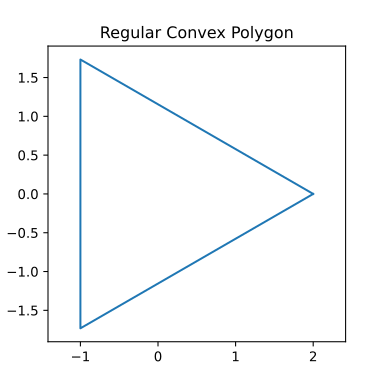
A regular polygon is a polygon that is direct equiangular (all angles are equal in measure) and equilateral (all sides have the same length). Regular polygons may be either convex, star or skew. In the limit, a sequence of regular polygons with an increasing number of sides approximates a circle.

\[r = \frac{a}{\cos \left(t - \alpha/2 - \alpha \ \lfloor \theta/\alpha \rfloor \right)}, \quad \text{where } \alpha = \frac{2 \pi}{n}.\]

\[x(t) = r \cos(t)),\]

\[y(t) = r \sin(t).\]

The Python code for the example below can be found online in the DataXlCalcNet repository or in the corresponding local DataXlCalcNet folder in the file D01_RegularConvexPolygon.py, and the XML code in the file D01_RegularConvexPolygon.2D.xml.

See also: https://en.wikipedia.org/wiki/Star_polygon

See also: https://mathcurve.com/polyedres/regulier/polygoneregulier.shtml

See also: https://mathcurve.com/courbes2d/goursat/goursat.shtml

See also: https://mathcurve.com/courbes3d.gb/polygramme/polygramme.shtml

See also: https://mathcurve.com/courbes3d.gb/billardcylindrique/billardcylindrique.shtml

Circle

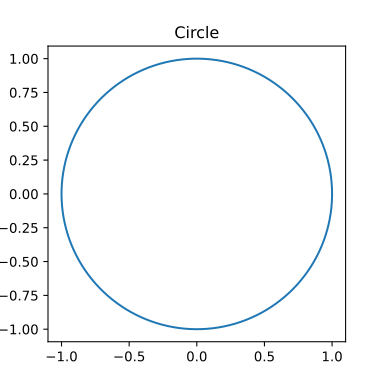
A circle is the set of points in a plane that are equidistant from a given point \(O\). The parametric equations for a circle of radius \(a\) can be given by

\[x(t) = a \cos(t)),\]

\[y(t) = a \sin(t).\]

See also Wikipedia [1368], MathWorld [1042], MathCurve [305].

The Python code for the example below can be found online in the DataXlCalcNet repository or in the corresponding local DataXlCalcNet folder in the file D02_Circle.py, and the XML code in the file D02_Circle.2D.xml.

Ellipse

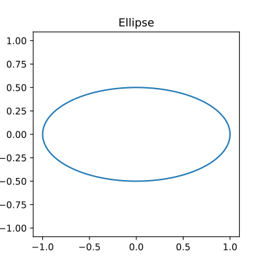
An ellipse is a plane curve surrounding two focal points, such that for all points on the curve, the sum of the two distances to the focal points is a constant. The parametric equations of a standard ellipse centered at the origin with width \(2a\) and height \(2b\) can be given by (with \(0 \le t < 2\pi\)):

\[x(t) = a \cos(t)),\]

\[y(t) = b \sin(t).\]

Assuming \(a \ge b\), the focal points are \((\pm \sqrt{a^2-b^2}, 0)\).

See also Wikipedia [1373], MathWorld [1044], MathCurve [307].

The Python code for the example below can be found online in the DataXlCalcNet repository or in the corresponding local DataXlCalcNet folder in the file D03_Ellipse.py, and the XML code in the file D03_Ellipse.2D.xml.

Parabola

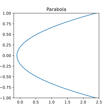
A parabola is a plane curve which is mirror-symmetrical and is approximately U-shaped. It fits several superficially different mathematical descriptions, which can all be proved to define exactly the same curves.

The graph of a quadratic function \(y = a x^2 + b x + c\) (with \(a \ne 0\)) is a parabola with its axis parallel to the \(y\)-axis. Conversely, every such parabola is the graph of a quadratic function.

The surface of revolution obtained by rotating a parabola about its axis of symmetry is called a paraboloid.

See also: https://mathworld.wolfram.com/Parabola.html

See also: https://en.wikipedia.org/wiki/Parabola

In polar coordinates, the equation of a parabola with parameter a and center (0, 0) is given by \(\displaystyle r(t) = - \frac{2a}{1 + \cos(t)}\). It can also be written parametrically as

\[x(t) = a t^2,\]

\[y(t) = 2 a t.\]

The Python code for the example below can be found online in the DataXlCalcNet repository or in the corresponding local DataXlCalcNet folder in the file D04_Parabola.py, and the XML code in the file D04_Parabola.2D.xml.

Hyperbola

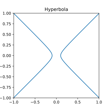
In polar coordinates, the equation of a hyperbola centered at the origin (i.e., with \(x_0=y_0=0\)) is \(\displaystyle r2(t) = \frac{a^2 b^2}{b^2 \cos^2(t) - a^2 \sin^2(t)}\).

Parametric equations for the right branch of a hyperbola are given by

\[x(t) = a \cosh(t),\]

\[y(t) = b \sinh(t),\]

which ranges over the right branch of the hyperbola.

A parametric representation which ranges over both branches of the hyperbola is

\[x(t) = a \sec(t),\]

\[y(t) = b \tan(t),\]

with \(t \in (-\pi,\pi)\) and discontinuities at \(\pm \pi/2\).

See also: https://mathworld.wolfram.com/Hyperbola.html

See also: https://mathworld.wolfram.com/ConicSection.html

The Python code for the example below can be found online in the DataXlCalcNet repository or in the corresponding local DataXlCalcNet folder in the file D05_Hyperbola.py, and the XML code in the file D05_Hyperbola.2D.xml.

Cycloid

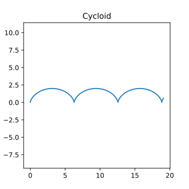
The cycloid is the locus of a point on the rim of a circle of radius a rolling along a straight line. If the cycloid has a cusp at the origin and its humps are oriented upward, its parametric equation is

\[x(t) = a (t - \sin(t)),\]

\[y(t) = a (t - \cos(t)).\]

See also Wikipedia [1372], MathWorld [1043], MathCurve [306].

The Python code for the example below can be found online in the DataXlCalcNet repository or in the corresponding local DataXlCalcNet folder in the file D06_Cycloid.py, and the XML code in the file D06_Cycloid.2D.xml.

Trochoid

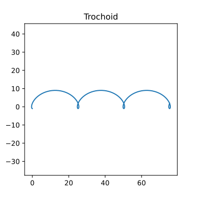
A trochoid is the locus of a point at a distance b from the center of a circle of radius a rolling on a fixed line. A trochoid has parametric equations

\[x(t) = a t - b \sin(t),\]

\[y(t) = a t - b \cos(t)).\]

If \(b<a\), the trochoid is known as a curtate cycloid; if \(b=a\), it is a cycloid; and if \(b>a\), the curve is a prolate cycloid.

See also Wikipedia [1396], MathWorld [1055], MathCurve [326].

The Python code for the example below can be found online in the DataXlCalcNet repository or in the corresponding local DataXlCalcNet folder in the file D07_Trochoid.py, and the XML code in the file D07_Trochoid.2D.xml.

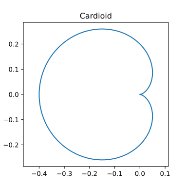
Cardioid

In geometry, a cardioid is a plane curve traced by a point on the perimeter of a circle that is rolling around a fixed circle of the same radius.

The polar equation is given by

\[r = a (1 - \cos (\theta)).\]

See also: Wikipedia [1401], MathWorld [1058]

The Python code for the example below can be found online in the DataXlCalcNet repository or in the corresponding local DataXlCalcNet folder in the file D08_Cardioid.py, and the XML code in the file D08_Cardioid.2D.xml.

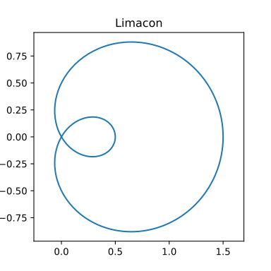
Limaçon curve

Returns the curve given by the polar equation

\[r = b + a \cos (\theta).\]

See also: see also Wikipedia [1415], MathWorld [1065]

The Python code for the example below can be found online in the DataXlCalcNet repository or in the corresponding local DataXlCalcNet folder in the file D09_LimaconCurve.py, and the XML code in the file D09_LimaconCurve.2D.xml.

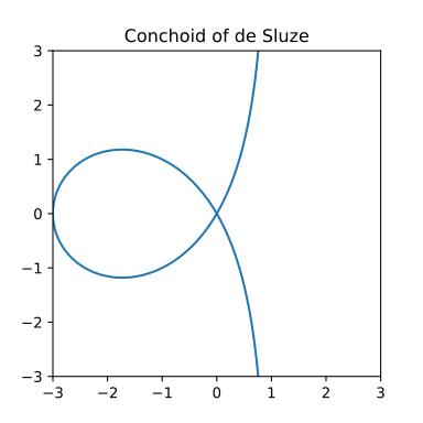
Conchoid of de Sluze

Returns the curve given by the polar equation

\[r = \sec(\theta) + a \cos (\theta).\]

See also: see also Wikipedia [1403], MathWorld [1059]

The Python code for the example below can be found online in the DataXlCalcNet repository or in the corresponding local DataXlCalcNet folder in the file D10_ConchoidOfDeSluze.py, and the XML code in the file D10_ConchoidOfDeSluze.2D.xml.

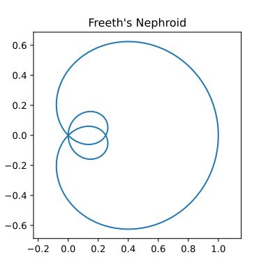
Freeth’s Nephroid

The curve has the polar equation

\[r = a \left[1 + 2 \sin \left(\tfrac{1}{2} \theta \right) \right]\]

See also: Wikipedia [1410], MathWorld [1063]

The Python code for the example below can be found online in the DataXlCalcNet repository or in the corresponding local DataXlCalcNet folder in the file D11_FreethNephroid.py, and the XML code in the file D11_FreethNephroid.2D.xml.

Strophoid

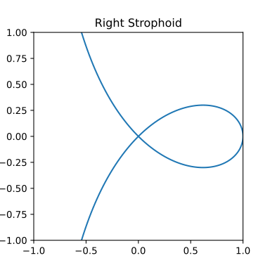
The name strophoid means “belt with a twist”. The polar form for a general strophoid is

\[r = \frac{b \sin(a - 2 \theta)}{\sin(a - \theta)}\]

See also: Wikipedia [1421], MathWorld [1069]

A special cases is the right strophoid with \(a = \pi/2\).

The Python code for the example below can be found online in the DataXlCalcNet repository or in the corresponding local DataXlCalcNet folder in the file D12_Strophoid.py, and the XML code in the file D12_Strophoid.2D.xml.

Cycloid of Ceva

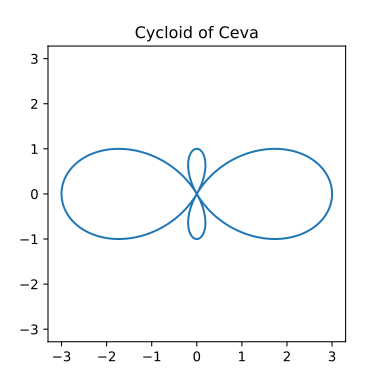
A curve with the polar form

\[r = 1 + 2 \cos(2 \theta).\]

See also: Wikipedia [1404], MathWorld [1060]

The Python code for the example below can be found online in the DataXlCalcNet repository or in the corresponding local DataXlCalcNet folder in the file D13_CycloidOfCeva.py, and the XML code in the file D13_CycloidOfCeva.2D.xml.

Lemniscate of Gerono

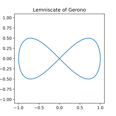
This curve is also known as Eight curve. It has parametric equations

\[x(t) = a \sin(t),\]

\[y(t) = x(t) \cos(t)).\]

See also Wikipedia [1387], MathWorld [1052], MathCurve [318].

The Python code for the example below can be found online in the DataXlCalcNet repository or in the corresponding local DataXlCalcNet folder in the file D14_LemniscateOfGerono.py, and the XML code in the file D14_LemniscateOfGerono.2D.xml.

Lemniscate of Bernoulli

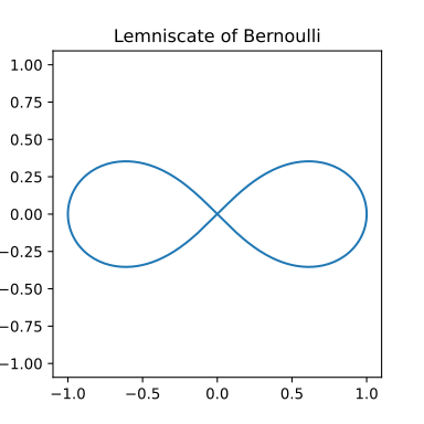
The lemniscate of Bernoulli is a polar curve defined as the locus of points such that the the product of distances from two fixed points \((-a,0)\) and \((a,0)\) is a constant \(a^2\). It has parametric equations

\[x(t) = \frac{a \cos(t)}{1 + \sin^2(t)},\]

\[y(t) = x(t) \sin(t)).\]

See also Wikipedia [1386], MathWorld [1051], MathCurve [317].

The Python code for the example below can be found online in the DataXlCalcNet repository or in the corresponding local DataXlCalcNet folder in the file D15_LemniscateOfBernoulli.py, and the XML code in the file D15_LemniscateOfBernoulli.2D.xml.