Introduction to 2D functions plots#
Simple plot of (well-behaved) functions in 2D#
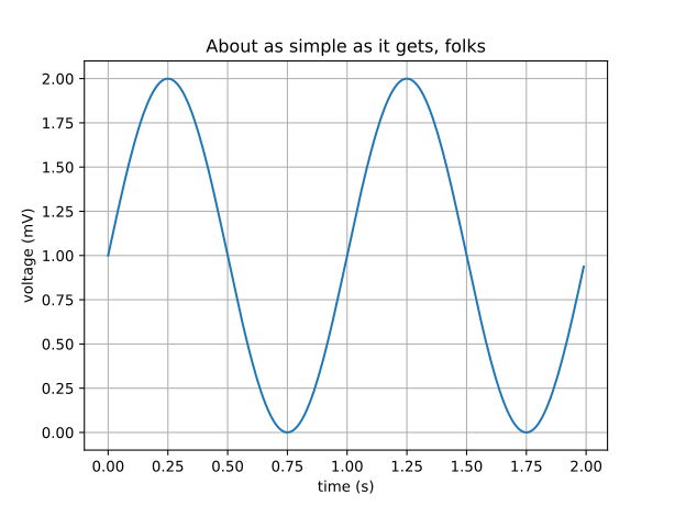
This is a (slightly modified) example from the Matplotlib tutorials.
See https://matplotlib.org/stable/gallery/lines_bars_and_markers/simple_plot.html
The Python code for the example below can be found online in the DataXlCalcNet repository or in the corresponding local DataXlCalcNet folder in the file D01_Simpleplot.py, and the XML code in the file D01_Simpleplot.2D.xml.
Function plots on different scales#
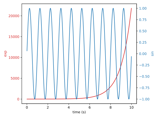
This is an example from the Matplotlib tutorials.
See https://matplotlib.org/stable/gallery/subplots_axes_and_figures/two_scales.html
The Python code for the example below can be found online in the DataXlCalcNet repository or in the corresponding local DataXlCalcNet folder in the file D02_PlotDiffScales.py, and the XML code in the file D02_PlotDiffScales.2D.xml.
Stepplot#
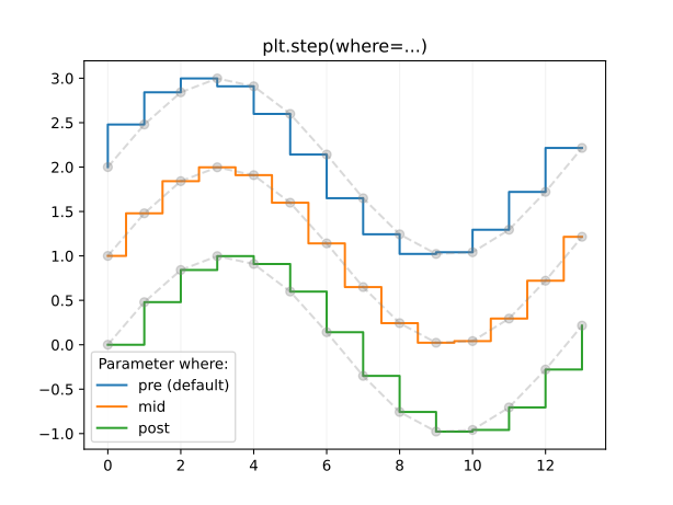
This is an example from the Matplotlib tutorials.
See https://matplotlib.org/stable/gallery/lines_bars_and_markers/step_demo.html
The Python code for the example below can be found online in the DataXlCalcNet repository or in the corresponding local DataXlCalcNet folder in the file D03_Stepplot.py, and the XML code in the file D03_Stepplot.2D.xml.
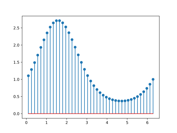
Stemplot#
This is an example from the Matplotlib tutorials.
The Python code for the example below can be found online in the DataXlCalcNet repository or in the corresponding local DataXlCalcNet folder in the file D04_Stemplot.py, and the XML code in the file D04_Stemplot.2D.xml.
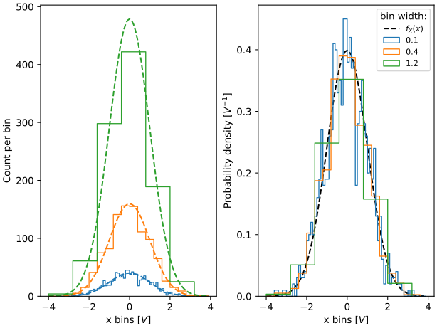
Histograms and densities#
This is an example from the Matplotlib tutorials.
See https://matplotlib.org/stable/gallery/statistics/histogram_normalization.html#
The Python code for the example below can be found online in the DataXlCalcNet repository or in the corresponding local DataXlCalcNet folder in the file D05_HistogramsAndDensities.py, and the XML code in the file D05_HistogramsAndDensities.2D.xml.
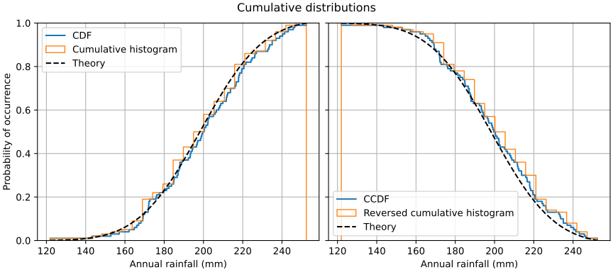
Cumulative histogram and CDF#
This is an example from the Matplotlib tutorials.
# see https://matplotlib.org/stable/gallery/statistics/histogram_cumulative.html#
The Python code for the example below can be found online in the DataXlCalcNet repository or in the corresponding local DataXlCalcNet folder in the file D06_CumulativeHistogramAndCDF.py, and the XML code in the file D06_CumulativeHistogramAndCDF.2D.xml.
Plots of continuous distribution functions#
Some text
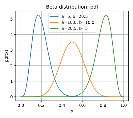
Probability density function (pdf)#
The Python code for the example below can be found online in the DataXlCalcNet repository or in the corresponding local DataXlCalcNet folder in the file D07_DistPlotContinuous.py, and the XML code in the file D07_DistPlotContinuous.2D.xml.
To produce the figure as shown below, the try-block at the end of the file should look like this:
try:
    if __name__ == '__main__':
        ylim = None
        target = 'pdf' # pdf, cdf, 'sf', 'hf', 'chf', 'qtf', 'isf'

        Title = 'Beta distribution'
        a = [5, 10.0, 20.5]
        b = [20.5, 10.0, 5]
        xlim = [0, 0.999]
        if target=='hf': ylim=[0, 100]

        dlist = []
        ltext = []
        for j in range(len(a)):
            dlist.append(dreal.dist_beta(a[j], b[j]))
            ltext.append('a=' + str(a[j]) + ', b=' + str(b[j]))

        DistPlotContinuous(Title = Title, dlist=dlist, xlim = xlim,
            ylim = ylim, target = target, ltext = ltext, marker='o',
            markersize=0)
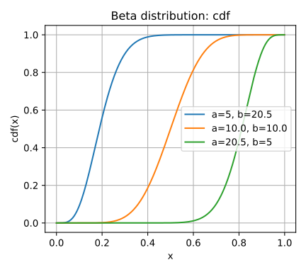
Cumulative distribution function (cdf)#
The Python code for the example below can be found online in the DataXlCalcNet repository or in the corresponding local DataXlCalcNet folder in the file D07_DistPlotContinuous.py, and the XML code in the file D07_DistPlotContinuous.2D.xml.
To produce the figure as shown below, the try-block at the end of the file should look like this:
try:
    if __name__ == '__main__':
        ylim = None
        target = 'cdf' # pdf, cdf, 'sf', 'hf', 'chf', 'qtf', 'isf'

        Title = 'Beta distribution'
        a = [5, 10.0, 20.5]
        b = [20.5, 10.0, 5]
        xlim = [0, 0.999]
        if target=='hf': ylim=[0, 100]

        dlist = []
        ltext = []
        for j in range(len(a)):
            dlist.append(dreal.dist_beta(a[j], b[j]))
            ltext.append('a=' + str(a[j]) + ', b=' + str(b[j]))

        DistPlotContinuous(Title = Title, dlist=dlist, xlim = xlim,
            ylim = ylim, target = target, ltext = ltext, marker='o',
            markersize=0)
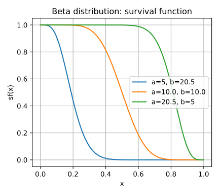
Survival function (sf)#
The Python code for the example below can be found online in the DataXlCalcNet repository or in the corresponding local DataXlCalcNet folder in the file D07_DistPlotContinuous.py, and the XML code in the file D07_DistPlotContinuous.2D.xml.
To produce the figure as shown below, the try-block at the end of the file should look like this:
try:
    if __name__ == '__main__':
        ylim = None
        target = 'sf' # pdf, cdf, 'sf', 'hf', 'chf', 'qtf', 'isf'

        Title = 'Beta distribution'
        a = [5, 10.0, 20.5]
        b = [20.5, 10.0, 5]
        xlim = [0, 0.999]
        if target=='hf': ylim=[0, 100]

        dlist = []
        ltext = []
        for j in range(len(a)):
            dlist.append(dreal.dist_beta(a[j], b[j]))
            ltext.append('a=' + str(a[j]) + ', b=' + str(b[j]))

        DistPlotContinuous(Title = Title, dlist=dlist, xlim = xlim,
            ylim = ylim, target = target, ltext = ltext, marker='o',
            markersize=0)
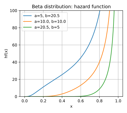
Hazard function (hf)#
The Python code for the example below can be found online in the DataXlCalcNet repository or in the corresponding local DataXlCalcNet folder in the file D07_DistPlotContinuous.py, and the XML code in the file D07_DistPlotContinuous.2D.xml.
To produce the figure as shown below, the try-block at the end of the file should look like this:
try:
    if __name__ == '__main__':
        ylim = None
        target = 'hf' # pdf, cdf, 'sf', 'hf', 'chf', 'qtf', 'isf'

        Title = 'Beta distribution'
        a = [5, 10.0, 20.5]
        b = [20.5, 10.0, 5]
        xlim = [0, 0.999]
        if target=='hf': ylim=[0, 100]

        dlist = []
        ltext = []
        for j in range(len(a)):
            dlist.append(dreal.dist_beta(a[j], b[j]))
            ltext.append('a=' + str(a[j]) + ', b=' + str(b[j]))

        DistPlotContinuous(Title = Title, dlist=dlist, xlim = xlim,
            ylim = ylim, target = target, ltext = ltext, marker='o',
            markersize=0)
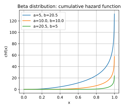
Cumulative hazard function (chf)#
The Python code for the example below can be found online in the DataXlCalcNet repository or in the corresponding local DataXlCalcNet folder in the file D07_DistPlotContinuous.py, and the XML code in the file D07_DistPlotContinuous.2D.xml.
To produce the figure as shown below, the try-block at the end of the file should look like this:
try:
    if __name__ == '__main__':
        ylim = None
        target = 'chf' # pdf, cdf, 'sf', 'hf', 'chf', 'qtf', 'isf'

        Title = 'Beta distribution'
        a = [5, 10.0, 20.5]
        b = [20.5, 10.0, 5]
        xlim = [0, 0.999]
        if target=='hf': ylim=[0, 100]

        dlist = []
        ltext = []
        for j in range(len(a)):
            dlist.append(dreal.dist_beta(a[j], b[j]))
            ltext.append('a=' + str(a[j]) + ', b=' + str(b[j]))

        DistPlotContinuous(Title = Title, dlist=dlist, xlim = xlim,
            ylim = ylim, target = target, ltext = ltext, marker='o',
            markersize=0)
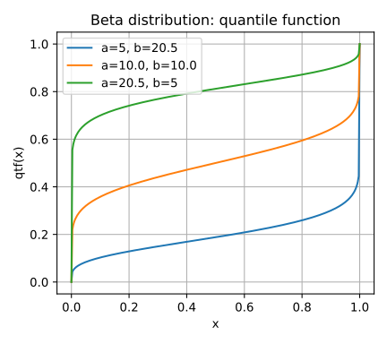
Quantile function (qtf)#
The Python code for the example below can be found online in the DataXlCalcNet repository or in the corresponding local DataXlCalcNet folder in the file D07_DistPlotContinuous.py, and the XML code in the file D07_DistPlotContinuous.2D.xml.
To produce the figure as shown below, the try-block at the end of the file should look like this:
try:
    if __name__ == '__main__':
        ylim = None
        target = 'qtf' # pdf, cdf, 'sf', 'hf', 'chf', 'qtf', 'isf'

        Title = 'Beta distribution'
        a = [5, 10.0, 20.5]
        b = [20.5, 10.0, 5]
        xlim = [0, 0.999]
        if target=='hf': ylim=[0, 100]

        dlist = []
        ltext = []
        for j in range(len(a)):
            dlist.append(dreal.dist_beta(a[j], b[j]))
            ltext.append('a=' + str(a[j]) + ', b=' + str(b[j]))

        DistPlotContinuous(Title = Title, dlist=dlist, xlim = xlim,
            ylim = ylim, target = target, ltext = ltext, marker='o',
            markersize=0)
Inverse survival function (isf)#
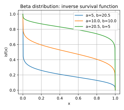
The Python code for the example below can be found online in the DataXlCalcNet repository or in the corresponding local DataXlCalcNet folder in the file D07_DistPlotContinuous.py, and the XML code in the file D07_DistPlotContinuous.2D.xml.
To produce the figure as shown below, the try-block at the end of the file should look like this:
try:
    if __name__ == '__main__':
        ylim = None
        target = 'qtf' # pdf, cdf, 'sf', 'hf', 'chf', 'qtf', 'isf'

        Title = 'Beta distribution'
        a = [5, 10.0, 20.5]
        b = [20.5, 10.0, 5]
        xlim = [0, 0.999]
        if target=='hf': ylim=[0, 100]

        dlist = []
        ltext = []
        for j in range(len(a)):
            dlist.append(dreal.dist_beta(a[j], b[j]))
            ltext.append('a=' + str(a[j]) + ', b=' + str(b[j]))

        DistPlotContinuous(Title = Title, dlist=dlist, xlim = xlim,
            ylim = ylim, target = target, ltext = ltext, marker='o',
            markersize=0)
Plots of discrete distribution functions#
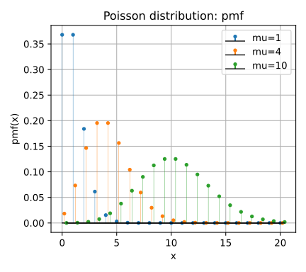
Probability mass function (pmf)#
The Python code for the example below can be found online in the DataXlCalcNet repository or in the corresponding local DataXlCalcNet folder in the file D08_DistPlotDiscrete.py, and the XML code in the file D08_DistPlotDiscrete.2D.xml.
To produce the figure as shown below, the try-block at the end of the file should look like this:
try:
    if __name__ == '__main__':
        ylim = None

        Title = 'Poisson distribution'
        target = 'pmf' # pmf, cdf, 'sf', 'hf', 'chf', 'qtf', 'isf'
        mu = [1, 4, 10]
        xlim = [0.0, 20.0]
        ylim = None
        if target=='qtf': ylim=[0, 20]

        dlist = []
        ltext = []
        for j in range(len(mu)):
            dlist.append(dreal.dist_poisson(mu[j]))
            ltext.append('mu=' + str(mu[j]))
        DistPlotDiscrete(Title = Title, dlist=dlist, xlim = xlim,  ylim = ylim,
            target = target, ltext = ltext, lattice=True, marker='o',
            markersize=3, vertical_lines=True)
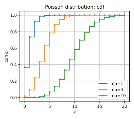
Cumulative distribution function (cdf)#
The Python code for the example below can be found online in the DataXlCalcNet repository or in the corresponding local DataXlCalcNet folder in the file D08_DistPlotDiscrete.py, and the XML code in the file D08_DistPlotDiscrete.2D.xml.
To produce the figure as shown below, the try-block at the end of the file should look like this:
try:
    if __name__ == '__main__':
        ylim = None

        Title = 'Poisson distribution'
        target = 'cdf' # pmf, cdf, 'sf', 'hf', 'chf', 'qtf', 'isf'
        mu = [1, 4, 10]
        xlim = [0.0, 20.0]
        ylim = None
        if target=='qtf': ylim=[0, 20]

        dlist = []
        ltext = []
        for j in range(len(mu)):
            dlist.append(dreal.dist_poisson(mu[j]))
            ltext.append('mu=' + str(mu[j]))
        DistPlotDiscrete(Title = Title, dlist=dlist, xlim = xlim,  ylim = ylim,
            target = target, ltext = ltext, lattice=True, marker='o',
            markersize=3, vertical_lines=True)
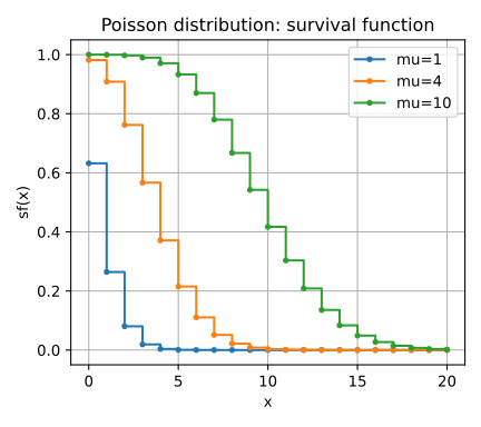
Survival function (sf)#
The Python code for the example below can be found online in the DataXlCalcNet repository or in the corresponding local DataXlCalcNet folder in the file D08_DistPlotDiscrete.py, and the XML code in the file D08_DistPlotDiscrete.2D.xml.
To produce the figure as shown below, the try-block at the end of the file should look like this:
try:
    if __name__ == '__main__':
        ylim = None

        Title = 'Poisson distribution'
        target = 'sf' # pmf, cdf, 'sf', 'hf', 'chf', 'qtf', 'isf'
        mu = [1, 4, 10]
        xlim = [0.0, 20.0]
        ylim = None
        if target=='qtf': ylim=[0, 20]

        dlist = []
        ltext = []
        for j in range(len(mu)):
            dlist.append(dreal.dist_poisson(mu[j]))
            ltext.append('mu=' + str(mu[j]))
        DistPlotDiscrete(Title = Title, dlist=dlist, xlim = xlim,  ylim = ylim,
            target = target, ltext = ltext, lattice=True, marker='o',
            markersize=3, vertical_lines=True)
Hazard function (hf)#
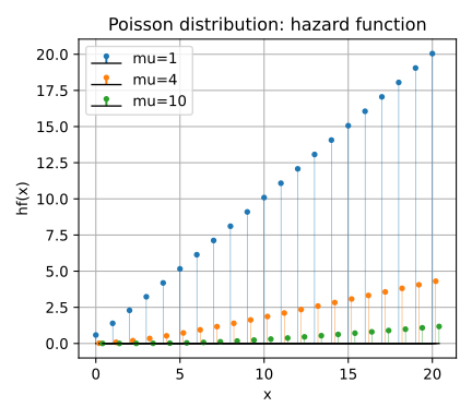
The Python code for the example below can be found online in the DataXlCalcNet repository or in the corresponding local DataXlCalcNet folder in the file D08_DistPlotDiscrete.py, and the XML code in the file D08_DistPlotDiscrete.2D.xml.
To produce the figure as shown below, the try-block at the end of the file should look like this:
try:
    if __name__ == '__main__':
        ylim = None

        Title = 'Poisson distribution'
        target = 'hf' # pmf, cdf, 'sf', 'hf', 'chf', 'qtf', 'isf'
        mu = [1, 4, 10]
        xlim = [0.0, 20.0]
        ylim = None
        if target=='qtf': ylim=[0, 20]

        dlist = []
        ltext = []
        for j in range(len(mu)):
            dlist.append(dreal.dist_poisson(mu[j]))
            ltext.append('mu=' + str(mu[j]))
        DistPlotDiscrete(Title = Title, dlist=dlist, xlim = xlim,  ylim = ylim,
            target = target, ltext = ltext, lattice=True, marker='o',
            markersize=3, vertical_lines=True)
Cumulative hazard function (chf)#
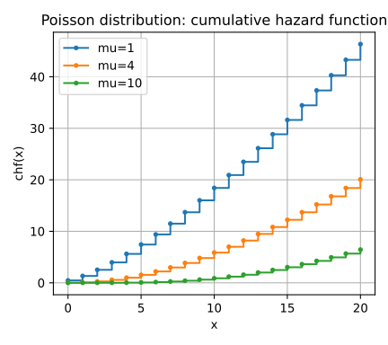
The Python code for the example below can be found online in the DataXlCalcNet repository or in the corresponding local DataXlCalcNet folder in the file D08_DistPlotDiscrete.py, and the XML code in the file D08_DistPlotDiscrete.2D.xml.
To produce the figure as shown below, the try-block at the end of the file should look like this:
try:
    if __name__ == '__main__':
        ylim = None

        Title = 'Poisson distribution'
        target = 'chf' # pmf, cdf, 'sf', 'hf', 'chf', 'qtf', 'isf'
        mu = [1, 4, 10]
        xlim = [0.0, 20.0]
        ylim = None
        if target=='qtf': ylim=[0, 20]

        dlist = []
        ltext = []
        for j in range(len(mu)):
            dlist.append(dreal.dist_poisson(mu[j]))
            ltext.append('mu=' + str(mu[j]))
        DistPlotDiscrete(Title = Title, dlist=dlist, xlim = xlim,  ylim = ylim,
            target = target, ltext = ltext, lattice=True, marker='o',
            markersize=3, vertical_lines=True)
Quantile function (qtf)#
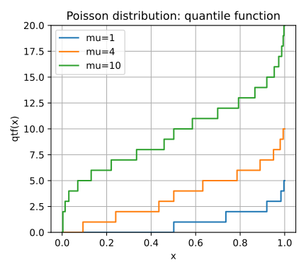
The Python code for the example below can be found online in the DataXlCalcNet repository or in the corresponding local DataXlCalcNet folder in the file D08_DistPlotDiscrete.py, and the XML code in the file D08_DistPlotDiscrete.2D.xml.
To produce the figure as shown below, the try-block at the end of the file should look like this:
try:
    if __name__ == '__main__':
        ylim = None

        Title = 'Poisson distribution'
        target = 'qtf' # pmf, cdf, 'sf', 'hf', 'chf', 'qtf', 'isf'
        mu = [1, 4, 10]
        xlim = [0.0, 20.0]
        ylim = None
        if target=='qtf': ylim=[0, 20]

        dlist = []
        ltext = []
        for j in range(len(mu)):
            dlist.append(dreal.dist_poisson(mu[j]))
            ltext.append('mu=' + str(mu[j]))
        DistPlotDiscrete(Title = Title, dlist=dlist, xlim = xlim,  ylim = ylim,
            target = target, ltext = ltext, lattice=True, marker='o',
            markersize=0, vertical_lines=True)
Inverse survival function (isf)#
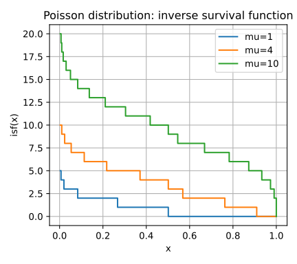
The Python code for the example below can be found online in the DataXlCalcNet repository or in the corresponding local DataXlCalcNet folder in the file D08_DistPlotDiscrete.py, and the XML code in the file D08_DistPlotDiscrete.2D.xml.
To produce the figure as shown below, the try-block at the end of the file should look like this:
try:
    if __name__ == '__main__':
        ylim = None

        Title = 'Poisson distribution'
        target = 'isf' # pmf, cdf, 'sf', 'hf', 'chf', 'qtf', 'isf'
        mu = [1, 4, 10]
        xlim = [0.0, 20.0]
        ylim = None
        if target=='qtf': ylim=[0, 20]

        dlist = []
        ltext = []
        for j in range(len(mu)):
            dlist.append(dreal.dist_poisson(mu[j]))
            ltext.append('mu=' + str(mu[j]))
        DistPlotDiscrete(Title = Title, dlist=dlist, xlim = xlim,  ylim = ylim,
            target = target, ltext = ltext, lattice=True, marker='o',
            markersize=0, vertical_lines=True)
Mpmath-inspired functions plots in 2D#
The plots discussed here show some possibilities to deal with not-so-well-behaved plots, i.e plots with real input, but (domain-wise) complex output, plots with singularities, and plots which grow very rapidly. The functions which are used here have been modified from Mpmath (see https://mpmath.readthedocs.io/en/stable/plotting.html).
These plots can use both Python-only contexts like mpm as well as FixedPrec contexts like math53, however, results may differ since the FixedPrec contexts enforce strict typing, whereas the Python-only contexts do not.
Simultaneous plot of sin and cos#
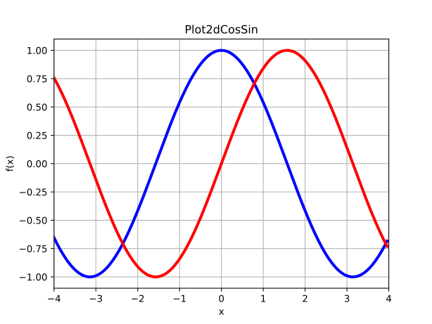
The Python code for the example below can be found online in the DataXlCalcNet repository or in the corresponding local DataXlCalcNet folder in the file D09_FuncPlot2d.py, and the XML code in the file D09_FuncPlot2d.2D.xml.
To produce the figure as shown below, using the mpm context, the try-block at the end of the file should look like this:
try:
    if __name__ == '__main__':
        FuncPlot2d(ctx=mpm, f=[mpm.cos, mpm.sin], xlim=[-4, 4],
            Title = 'Plot2dCosSin')
To produce the figure as shown below, using the math53 context, the try-block at the end of the file should look like this:
try:
    if __name__ == '__main__':
        FuncPlot2d(ctx=math53, f=[ctx.cos, ctx.sin], xlim=[-4, 4],
            Title = 'Plot2dCosSin')
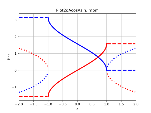
Simultaneous plots of asin and acos, for mpm and math53#
The Python code for the example below can be found online in the DataXlCalcNet repository or in the corresponding local DataXlCalcNet folder in the file D09_FuncPlot2d.py.
To produce the figure as shown below, using the mpm context, the try-block at the end of the file should look like this:
try:
    if __name__ == '__main__':
        FuncPlot2d(ctx=mpm, f=[mpm.acos, mpm.asin], xlim=[-2, 2],
            Title = 'Simultaneous plot of asin an acos, using mpm')
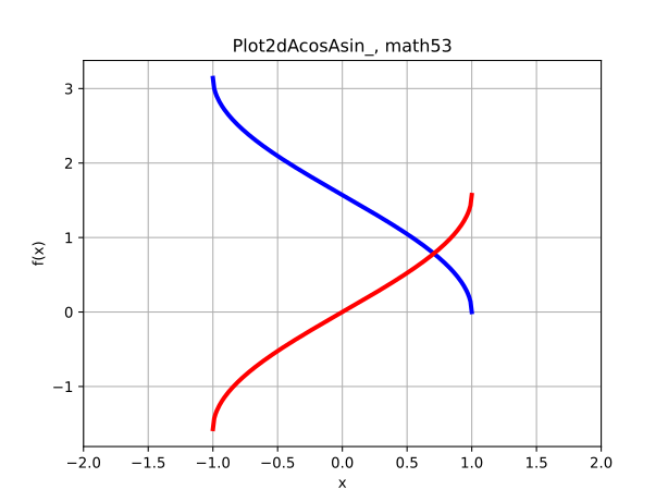
To produce the figure as shown below, the try-block at the end of the file should look like this:
try:
    if __name__ == '__main__':
        FuncPlot2d(ctx=math53, f=[ctx.acos, ctx.asin], xlim=[-2, 2],
            Title = 'Simultaneous plot of asin and acos, using math53')
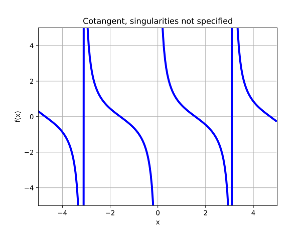
Plot of cotangent without singularities specified#
The Python code for the example below can be found online in the DataXlCalcNet repository or in the corresponding local DataXlCalcNet folder in the file D09_FuncPlot2d.py.
If we plot the cotangent without specifying the singularities, we get the results shown below:
To produce the left figure as shown below, the try-block at the end of the file should look like this:
try:
    if __name__ == '__main__':
        FuncPlot2d(ctx=mpm, f=mpm.cot, xlim=[-5, 5], ylim=[-5, 5],
            Title = 'Cotangent, singularities not specified, Mpm')
To produce the right figure as shown below, the try-block at the end of the file should look like this:
try:
    if __name__ == '__main__':
        FuncPlot2d(ctx=math53, f=ctx.cot, xlim=[-5, 5], ylim=[-5, 5],
            Title = 'Cotangent, singularities not specified, Math53')
Plot of cotangent with singularities specified#
The Python code for the example below can be found online in the DataXlCalcNet repository or in the corresponding local DataXlCalcNet folder in the file D09_FuncPlot2d.py.
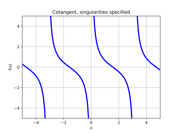
If we plot the cotangent and specify the singularities, we get the results shown below:
To produce the left figure as shown below, the try-block at the end of the file should look like this:
try:
    if __name__ == '__main__':
        FuncPlot2d(ctx=mpm, f=mpm.cot, xlim=[-5, 5], ylim=[-5, 5],
            singularities=[-mpm.pi, 0, mpm.pi],
            Title = 'Cotangent, singularities specified, mpm')
To produce the right figure as shown below, the try-block at the end of the file should look like this:
try:
    if __name__ == '__main__':
        FuncPlot2d(ctx=math53, f=ctx.cot, xlim=[-5, 5], ylim=[-5, 5],
            singularities=[-ctx.pi(), 0, ctx.pi()],
            Title = 'Cotangent, singularities specified, math53')