Roots and quadratic, cubic, and quartic equations

Square root, \(\mathrm{sqrt}(x) = \sqrt{x}\)

ctx.sqrt(x)

where ctx is math53, mathc53, ctxcpp, ctxflint.

Returns the principal square root of \(x\), \(\sqrt x\). See also Wikipedia [1352], MathWorld [930], Flint [811], Ehrhardt [309] (4.1.19), Mpmath [585].

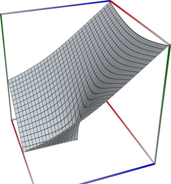
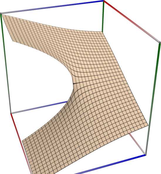
For positive real numbers, the principal root is simply the positive square root. For arbitrary complex numbers, the principal square root is defined to satisfy \(\sqrt x = \exp(\log(x)/2)\). The function thus has a branch cut along the negative half real axis.

\(\quad\) \(\quad\)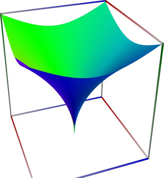

Left figure: real part of the Sqrt function. Camera angles are \(\theta=135^\circ\) and \(\phi = -12^\circ\), camera radius is -2.

Middle figure: imaginary part of the Sqrt function. Camera angles are \(\theta=135^\circ\) and \(\phi = -12^\circ\), camera radius is -2.

Right figure: absolute value of the Sqrt function, with color-coded phase. Camera angles are \(\theta=135^\circ\) and \(\phi = -12^\circ\), camera radius is -2.

An example in Python

>>> from xlcalcnet import xreal
>>> xreal.Sqrt(0.5)
xreal('5.2359877559829887307E-1')
>>> xreal.Sqrt('0.51')
xreal('5.3518479027559984754E-1')

An example in Visual Basic

>>> from xlcalcnet import Gpr
>>> Gpr.Sqrt(0.5)
Gpr('5.2359877559829887307E-1')
>>> Gpr.Sqrt('0.51')
Gpr('5.3518479027559984754E-1')

An example with real input:

>>> from xlcalcnet import dec, mpm, ipm
>>> mpm.dps = 40; x = '10.7'
>>> \mathrm{d}x = dec.sqrt(x); mx = mpm.sqrt(x); ix = ipm.sqrt(x)
>>> mpm.show([\mathrm{d}x, mx, ix])
dec:  3.271085446759225212153564923603401085326E+0
mpm:  3.271085446759225212153564923603401085326e+0
ipm:  3.271085446759225212153564923603401085326e+0 (7.019e-40%)

>>> from xlcalcnet import mpm, fpm, gmp, apm
>>> mpm.dps = 40; x = '10.7'
>>> fx = fpm.sqrt(x); gx = gmp.sqrt(x); ax = apm.sqrt(x)
>>> mpm.show([fx, gx, ax])
fpm:  3.27108544675922E+00
gmp:  3.271085446759225212153564923603401085326E+00
apm:  3.271085446759225212153564923603401085326e+0 (7.019e-40%)

The following example with complex input shows that the relative error can be high in double precision:

>>> from xlcalcnet import dec, mpm, ipm
>>> mpm.dps = 20; z = '10.2 + 1.5E-2j'
>>> \mathrm{d}z = dec.sqrt(z); mz = mpm.sqrt(z); iz = ipm.sqrt(z)
>>> mpm.show([\mathrm{d}z, mz, iz], aligned=True)
dec: 3.1937447478943743524E+0              + 2.3483404567458704692E-3j
mpm: 3.1937447478943743524e+0              + 2.3483404567458704692e-3j
ipm: 3.1937447478943743524e+0 (5.304e-20%) + 2.3483404567458704692e-3 (2.113e-19%)j

>>> from xlcalcnet import mpm, fpm, gmp, apm
>>> mpm.dps = 20; z = '10.2 + 1.5E-2j'
>>> fz = fpm.sqrt(z); gz = gmp.sqrt(z); az = apm.sqrt(z)
>>> mpm.show([fz, gz, az], aligned=True)
fpm: 3.19374474789437E+00                  + 2.34834045674587E-03j
gmp: 3.1937447478943743524E+00             + 2.3483404567458704692E-03j
apm: 3.1937447478943743524e+0 (1.061e-19%) + 2.3483404567458704692e-3 (1.409e-19%)j

Reciprocal square root, \(\mathrm{rsqrt}(x) = 1/\sqrt{x}\)

ctx.rsqrt(x)

where ctx is math53, mathc53, ctxcpp, ctxflint.

Returns the reciprocal of the principal square root of \(x\), \(1/\sqrt x\). See also Wikipedia [1352], MathWorld [930], Flint [811], Ehrhardt [309] (4.1.19), Mpmath [585].

An example in Python

>>> from xlcalcnet import xreal
>>> xreal.Rsqrt(0.5)
xreal('5.2359877559829887307E-1')
>>> xreal.Rsqrt('0.51')
xreal('5.3518479027559984754E-1')

An example in Visual Basic

>>> from xlcalcnet import Gpr
>>> Gpr.Rsqrt(0.5)
Gpr('5.2359877559829887307E-1')
>>> Gpr.Rsqrt('0.51')
Gpr('5.3518479027559984754E-1')

An example with real input:

>>> from xlcalcnet import dec, mpm, ipm
>>> mpm.dps = 40; x = '10.7'
>>> \mathrm{d}x = dec.RSqrt(x); mx = mpm.RSqrt(x); ix = ipm.RSqrt(x)
>>> mpm.show([\mathrm{d}x, mx, ix])
dec:  3.271085446759225212153564923603401085326E+0
mpm:  3.271085446759225212153564923603401085326e+0
ipm:  3.271085446759225212153564923603401085326e+0 (7.019e-40%)

>>> from xlcalcnet import mpm, fpm, gmp, apm
>>> mpm.dps = 40; x = '10.7'
>>> fx = fpm.RSqrt(x); gx = gmp.RSqrt(x); ax = apm.RSqrt(x)
>>> mpm.show([fx, gx, ax])
fpm:  3.27108544675922E+00
gmp:  3.271085446759225212153564923603401085326E+00
apm:  3.271085446759225212153564923603401085326e+0 (7.019e-40%)

The following example with complex input shows that the relative error can be high in double precision:

>>> from xlcalcnet import dec, mpm, ipm
>>> mpm.dps = 20; z = '10.2 + 1.5E-2j'
>>> \mathrm{d}z = dec.RSqrt(z); mz = mpm.RSqrt(z); iz = ipm.RSqrt(z)
>>> mpm.show([\mathrm{d}z, mz, iz], aligned=True)
dec: 3.1937447478943743524E+0              + 2.3483404567458704692E-3j
mpm: 3.1937447478943743524e+0              + 2.3483404567458704692e-3j
ipm: 3.1937447478943743524e+0 (5.304e-20%) + 2.3483404567458704692e-3 (2.113e-19%)j

>>> from xlcalcnet import mpm, fpm, gmp, apm
>>> mpm.dps = 20; z = '10.2 + 1.5E-2j'
>>> fz = fpm.RSqrt(z); gz = gmp.RSqrt(z); az = apm.RSqrt(z)
>>> mpm.show([fz, gz, az], aligned=True)
fpm: 3.19374474789437E+00                  + 2.34834045674587E-03j
gmp: 3.1937447478943743524E+00             + 2.3483404567458704692E-03j
apm: 3.1937447478943743524e+0 (1.061e-19%) + 2.3483404567458704692e-3 (1.409e-19%)j

Auxiliary function \(\mathrm{sqrt1pm1}(x) = \sqrt{1+x}-1\)

ctx.sqrt1pm1(x)

where ctx is math53, mathc53, ctxcpp , ctxboost or ctxflint.

Returns \(\sqrt{1+x}-1\), accurate also for \(x\) near 0. See also Wikipedia [1352], MathWorld [930], BoostMath [98].

This is calculated as \(\mathrm{sqrt1pm1}(v) = \mathrm{expm1}(\mathrm{logp1}(v)/2)\). See log1p() and expm1().

An example in Python

>>> from xlcalcnet import xreal
>>> xreal.Sqrt1pm1(0.5)
xreal('5.2359877559829887307E-1')
>>> xreal.Sqrt1pm1('0.51')
xreal('5.3518479027559984754E-1')

An example in Visual Basic

>>> from xlcalcnet import Gpr
>>> Gpr.Sqrt1pm1(0.5)
Gpr('5.2359877559829887307E-1')
>>> Gpr.Sqrt1pm1('0.51')
Gpr('5.3518479027559984754E-1')

An example with real input:

>>> from xlcalcnet import dec, mpm, ipm
>>> mpm.dps = 40; x = '1.0E-10'
>>> \mathrm{d}x = dec.sqrt1pm1(x); mx = mpm.sqrt1pm1(x); ix = ipm.sqrt1pm1(x)
>>> mpm.show([\mathrm{d}x, mx, ix])
dec:  4.999999999875000000006249999999609375000E-11
mpm:  4.999999999875000000006249999999609375000e-11
ipm:  4.999999999875000000006249999999609597867e-11 (1.121e-32%)

>>> from xlcalcnet import mpm, fpm, gmp, apm
>>> mpm.dps = 40; x = '1.0E-10'
>>> fx = fpm.sqrt1pm1(x); gx = gmp.sqrt1pm1(x); ax = apm.sqrt1pm1(x)
>>> mpm.show([fx, gx, ax])
fpm:  4.99999999987500E-11
gmp:  4.999999999875000000006249999999609375000E-11
apm:  4.999999999875000000006249999999609375000e-11 (1.336e-39%)

The following example with complex input shows that the relative error can be high in double precision:

>>> from xlcalcnet import dec, mpm, ipm
>>> mpm.dps = 20; z = '1.0E-10+ 1.5E-12j'
>>> \mathrm{d}z = dec.sqrt1pm1(z); mz = mpm.sqrt1pm1(z); iz = ipm.sqrt1pm1(z)
>>> mpm.show([\mathrm{d}z, mz, iz], aligned=True)
dec: 4.9999999998750281250E-11              + 7.4999999996250000000E-13j
mpm: 4.9999999998750281250e-11              + 7.4999999996250000000e-13j
ipm: 4.9999999998750315383e-11 (8.272e-13%) + 7.4999999996250000000e-13 (1.541e-19%)j

>>> from xlcalcnet import mpm, fpm, gmp, apm
>>> mpm.dps = 20; z = '1.0E-10+ 1.5E-12j'
>>> fz = fpm.sqrt1pm1(z); gz = gmp.sqrt1pm1(z); az = apm.sqrt1pm1(z)
>>> mpm.show([fz, gz, az], aligned=True)
fpm: 4.99999999987503E-11                   + 7.49999999962500E-13j
gmp: 4.9999999998750281250E-11              + 7.4999999996250000000E-13j
apm: 4.9999999998750281250e-11 (1.972e-19%) + 7.4999999996250000000e-13 (2.054e-19%)j

Cube root, \(\mathrm{cbrt}(x) = \sqrt[3]{x}\)

ctx.cbrt(x)

where ctx is math53, mathc53, ctxcpp, ctxboost, ctxflint.

Returns the cube root of \(x\), \(x^{1/3}\). See also Wikipedia [1339], MathWorld [915], BoostMath [103], Ehrhardt [309] (4.2.17), Mpmath [568].

This function is faster and more accurate than raising to a floating-point fraction.

An example in Python

>>> from xlcalcnet import xreal
>>> xreal.Cbrt(0.5)
xreal('5.2359877559829887307E-1')
>>> xreal.Cbrt('0.51')
xreal('5.3518479027559984754E-1')

An example in Visual Basic

>>> from xlcalcnet import Gpr
>>> Gpr.Cbrt(0.5)
Gpr('5.2359877559829887307E-1')
>>> Gpr.Cbrt('0.51')
Gpr('5.3518479027559984754E-1')

An example with real input:

>>> from xlcalcnet import dec, mpm, ipm
>>> mpm.dps = 40; x = '10.7'
>>> \mathrm{d}x = dec.cbrt(x); mx = mpm.cbrt(x); ix = ipm.cbrt(x)
>>> mpm.show([\mathrm{d}x, mx, ix])
dec:  2.203575453221625471351673513142748323963E+0
mpm:  2.203575453221625471351673513142748323963e+0
ipm:  2.203575453221625471351673513142748323963e+0 (1.042e-39%)

>>> from xlcalcnet import mpm, fpm, gmp, apm
>>> mpm.dps = 40; x = '10.7'
>>> fx = fpm.cbrt(x); gx = gmp.cbrt(x); ax = apm.cbrt(x)
>>> mpm.show([fx, gx, ax])
fpm:  2.20357545322163E+00
gmp:  2.203575453221625471351673513142748323963E+00
apm:  2.203575453221625471351673513142748323963e+0 (1.042e-39%)

The following example with complex input shows that the relative error can be high in double precision:

>>> from xlcalcnet import dec, mpm, ipm
>>> mpm.dps = 20; z = '10.2 + 1.5E-2j'
>>> \mathrm{d}z = dec.cbrt(z); mz = mpm.cbrt(z); iz = ipm.cbrt(z)
>>> mpm.show([\mathrm{d}z, mz, iz], aligned=True)
dec: 2.1687034063721566890E+0              + 1.0630892238793233640E-3j
mpm: 2.1687034063721566890e+0              + 1.0630892238793233640e-3j
ipm: 2.1687034063721566890e+0 (7.811e-20%) + 1.0630892238793233640e-3 (3.112e-19%)j

>>> from xlcalcnet import mpm, fpm, gmp, apm
>>> mpm.dps = 20; z = '10.2 + 1.5E-2j'
>>> fz = fpm.cbrt(z); gz = gmp.cbrt(z); az = apm.cbrt(z)
>>> mpm.show([fz, gz, az], aligned=True)
fpm: 2.16870340637216E+00                  + 1.06308922387932E-03j
gmp: 2.1687034063721566890E+00             + 1.0630892238793233640E-03j
apm: 2.1687034063721566890e+0 (7.811e-20%) + 1.0630892238793233640e-3 (2.334e-19%)j

Every nonzero complex number has three cube roots. This function returns the cube root defined by \(\exp(\log(x)/3)\) where the principal branch of the natural logarithm is used. Note that this does not give a real cube root for negative real numbers:

>>> mp.pretty = True
>>> mp.cbrt(-1)
(0.5 + 0.866025403784439j)

If you want the real cube root for negative real numbers, use the function cuberoot instead.

Nth root, \(\mathrm{nroot}(x, n) = \sqrt[n]{x}\)

ctx.nroot(x, n, k=0)

where ctx is math53, mathc53, ctxcpp or ctxflint.

Returns the nth root of \(x\). For real negative \(x\), \(n\) needs to be an odd integer for a real result. See also Wikipedia [1389], MathWorld [1011], Flint [811], Flint [801], Ehrhardt [309] (4.2.47), Mpmath [651].

See also: https://dlmf.nist.gov/1.11#iv

The roots of \(z^n = a + ib\) are

\[\sqrt[n]{R}\left(\cos\left(\frac{\alpha+2k\pi}{n}\right)+i\sin\left(\frac{\alpha+2k\pi}{n}\right)\right),\]

where \(\displaystyle R = \sqrt{a^2 + b^2}, \alpha = \mathrm{ph}(a + ib)\), with the principal value phase, and \(k = 0,1,\ldots,n-1\).

An example in Python

>>> from xlcalcnet import xreal
>>> xreal.Nroot(0.5, 4)
xreal('5.2359877559829887307E-1')
>>> xreal.Nroot('0.51', 4)
xreal('5.3518479027559984754E-1')

An example in Visual Basic

>>> from xlcalcnet import Gpr
>>> Gpr.Nroot(0.5, 4)
Gpr('5.2359877559829887307E-1')
>>> Gpr.Nroot('0.51', 4)
Gpr('5.3518479027559984754E-1')

An example with real input:

>>> from xlcalcnet import dec, mpm, ipm
>>> mpm.dps = 40; x = '125'; n = '3'
>>> \mathrm{d}x = dec.nthroot(x, n); mx = mpm.nthroot(x, n); ix = ipm.nthroot(x, n)
>>> mpm.show([\mathrm{d}x, mx, ix])
dec:  5.000000000000000000000000000000000000000E+0
mpm:  5.000000000000000000000000000000000000000e+0
ipm:  5.000000000000000000000000000000000000000e+0 (2.755e-39%)

>>> from xlcalcnet import mpm, fpm, gmp, apm
>>> mpm.dps = 40; x = '125'; n = '3'
>>> fx = fpm.nthroot(x, n); gx = gmp.nthroot(x, n); ax = apm.nthroot(x, n)
>>> mpm.show([fx, gx, ax])
fpm:  5.00000000000000E+00
gmp:  5.000000000000000000000000000000000000000E+00
apm:  5.000000000000000000000000000000000000002e+0 (3.673e-39%)

The following example with complex input shows that the relative error can be high in double precision:

>>> from xlcalcnet import dec, mpm, ipm
>>> mpm.dps = 20; z = '20.2 + 1.5E-2j'; n = '3'
>>> \mathrm{d}z = dec.nthroot(z, n); mz = mpm.nthroot(z, n); iz = ipm.nthroot(z, n)
>>> mpm.show([\mathrm{d}z, mz, iz], aligned=True)
dec: 2.7234358484296702080E+0              + 6.7411767412563680216E-4j
mpm: 2.7234358484296702080e+0              + 6.7411767412563680216e-4j
ipm: 2.7234358484296702080e+0 (1.866e-19%) + 6.7411767412563680216e-4 (4.295e-19%)j

>>> from xlcalcnet import mpm, fpm, gmp, apm
>>> mpm.dps = 20; z = '20.2 + 1.5E-2j'; n = '3'
>>> fz = fpm.nthroot(z, n); gz = gmp.nthroot(z, n); az = apm.nthroot(z, n)
>>> mpm.show([fz, gz, az], aligned=True)
fpm: 2.72343584842967E+00                  + 6.74117674125637E-04j
gmp: 2.7234358484296702080E+00             + 6.7411767412563680216E-04j
apm: 2.7234358484296702081e+0 (4.354e-19%) + 6.7411767412563680216e-4 (6.135e-19%)j

Unit root, \(\mathrm{unitroot}(n)\)

ctx.unitroot(n)

where ctx is math53, mathc53, ctxcpp or ctxflint.

Returns the nth root of z.

See also Wikipedia [1396], MathWorld [1006], Mpmath [650].

Caution

This still needs to be implemented

An example in Python

>>> from xlcalcnet import XComplex
>>> XComplex.Unitroots(0.5)
XComplex('5.2359877559829887307E-1')
>>> XComplex.Unitroots('0.1')
XComplex('5.3518479027559984754E-1')

An example in Visual Basic

>>> from xlcalcnet import Gpc
>>> Gpc.Unitroots(0.5)
Gpc('5.2359877559829887307E-1')
>>> Gpc.Unitroots('0.1')
Gpc('5.3518479027559984754E-1')