Lerch’s transcendent and Lerch’s zeta

Lerch’s transcendent, \(\Phi(x,s,a)\)

ctx.lerch_phi(s, z, a)

where ctx is math53 or ctxflint.

Returns the Lerch transcendent \(\Phi(z, s, a)\). See also Wikipedia [1469], MathWorld [1082], NIST [13], Ehrhardt [309] (3.6.10), Flint [834], Mpmath [738].

The function is defined for \(|z| < 1\) and \(\Re{a} > 0\) by

\[\Phi(z,s,a) = \sum_{k=0}^{\infty} \frac{z^k}{(a+k)^s}\]

and generally by the recurrence \(\Phi(z,s,a) = z \Phi(z,s,a+1) + a^{-s}\) along with the integral representation valid for \(\Re{a} > 0\)

\[\Phi(z,s,a) = \frac{1}{2 a^s} + \int_0^{\infty} \frac{z^t}{(a+t)^s} \mathrm{d}t - 2 \int_0^{\infty} \frac{\sin(t \log z - s \mathrm{arctan}(t/a)}{(a^2 + t^2)^{s/2} (e^{2 \pi t}-1)} \mathrm{d}t.\]

The Amath implementation requires \(x \le 1, s \ge -1, a \ge 0\). We have also \(\Phi(x,0,a) = 1/(1-x)\) and \(\Phi(x,s,0) = \text{Li}_s(x)\).

See also: https://fredrikj.net/blog/2022/02/computing-the-lerch-transcendent/

\(\quad\) \(\quad\)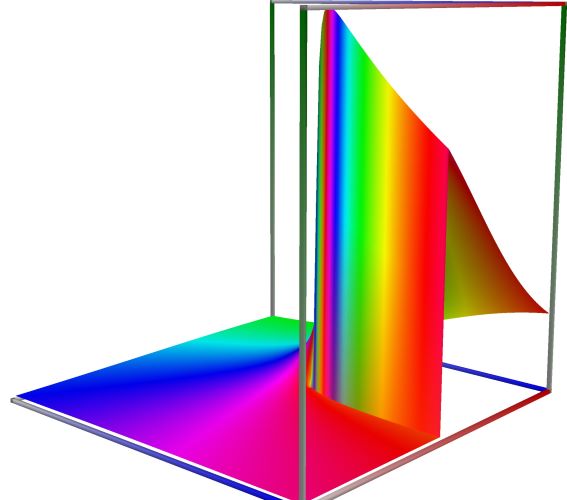

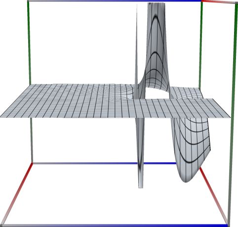
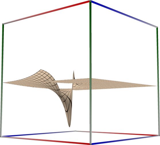
Left figure: real part of Lerch’s phi. Camera angles are \(\theta=135^\circ\) and \(\phi = -12^\circ\), camera radius is -2.

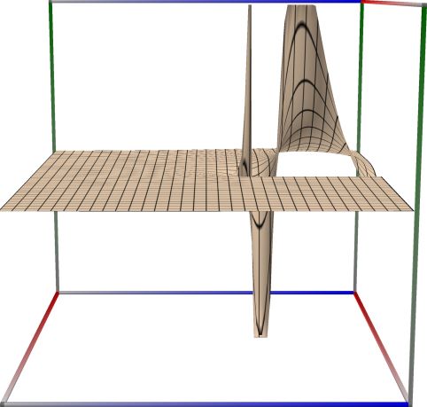
Middle figure: imaginary part of Lerch’s phi. Camera angles are \(\theta=135^\circ\) and \(\phi = -12^\circ\), camera radius is -2.

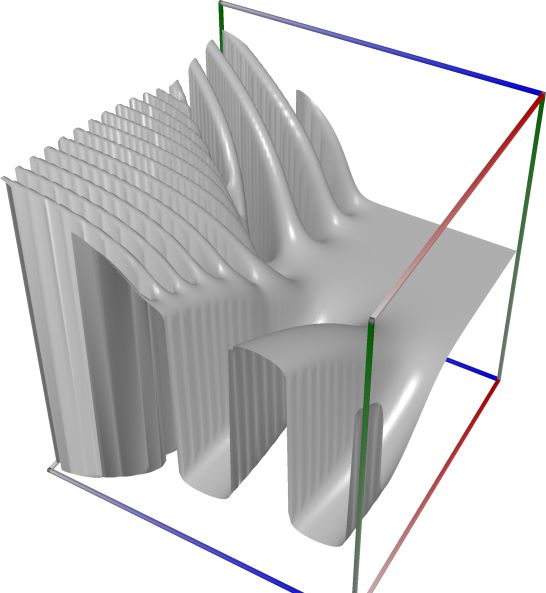
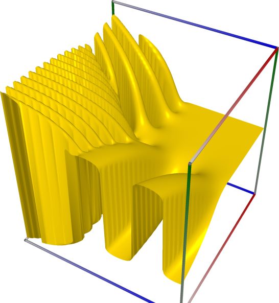
Right figure: absolute value of Lerch’s phi, with color-coded phase. Camera angles are \(\theta=135^\circ\) and \(\phi = -12^\circ\), camera radius is -2.

\(\quad\) \(\quad\)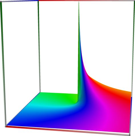

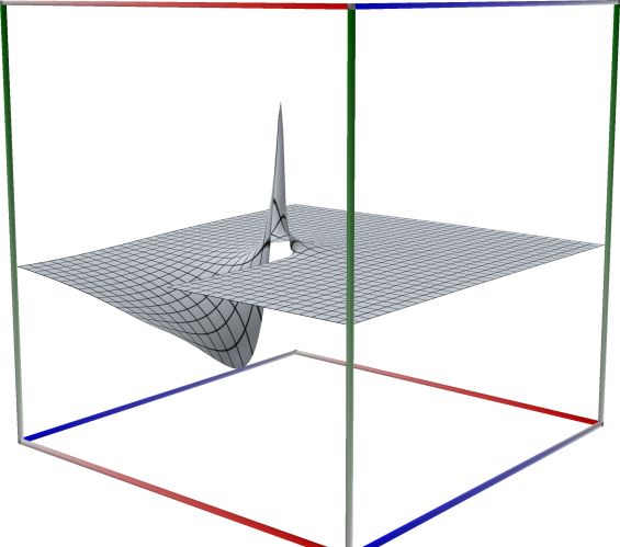
Left figure: real part of Lerch’s phi. Camera angles are \(\theta=135^\circ\) and \(\phi = -12^\circ\), camera radius is -2.

Middle figure: imaginary part of Lerch’s phi. Camera angles are \(\theta=135^\circ\) and \(\phi = -12^\circ\), camera radius is -2.

Right figure: absolute value of Lerch’s phi, with color-coded phase. Camera angles are \(\theta=135^\circ\) and \(\phi = -12^\circ\), camera radius is -2.

\(\quad\) \(\quad\)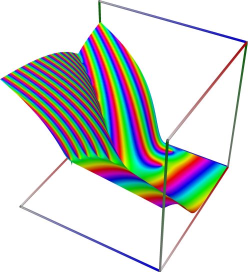

Left figure: real part of Lerch’s phi. Camera angles are \(\theta=135^\circ\) and \(\phi = -12^\circ\), camera radius is -2.

Middle figure: imaginary part of Lerch’s phi. Camera angles are \(\theta=135^\circ\) and \(\phi = -12^\circ\), camera radius is -2.

Right figure: absolute value of Lerch’s phi, with color-coded phase. Camera angles are \(\theta=135^\circ\) and \(\phi = -12^\circ\), camera radius is -2.

An example in Python

>>> from xlcalcnet import xreal
>>> xreal.LerchPhi(2,5, 0.5, 3)
xreal('5.2359877559829887307E-1')
>>> xreal.LerchPhi('5.1', 0.5, 3)
xreal('5.3518479027559984754E-1')

An example in Visual Basic

>>> from xlcalcnet import Gpr
>>> Gpr.LerchPhi(2,5, 0.5, 3)
Gpr('5.2359877559829887307E-1')
>>> Gpr.LerchPhi('5.1', 0.5, 3)
Gpr('5.3518479027559984754E-1')

An example with real input, \(x=1\) (same result as Hurwitz zeta):

>>> from xlcalcnet import dec, mpm, gmp, fpm, apm
>>> mpm.dps = 40; x = '1.0'; s = '2.5'; a = '3.0'
>>> \mathrm{d}x = dec.lerchphi(x, s, a); mx = mpm.lerchphi(x, s, a); gx = gmp.lerchphi(x, s, a)
>>> fx = fpm.lerchphi(x, s, a); ax = apm.lerchphi(x, s, a)
>>> mpm.show([\mathrm{d}x, mx, gx, fx, ax], aligned=True)
dec: 1.647105619542802986565586028223998768018E-1
mpm: 1.647105619542802986565586028223998768018e-1
gmp: 1.647105619542802986565586028223998768018E-01
fpm: 1.64710561954280E-01
apm: 1.647105619542802986565586028223998768018e-1 (1.742e-39%)

An example with real input, \(x<1, s \geq 0, a>0\) (real result for real \(x, s, a\)):

>>> from xlcalcnet import dec, mpm, gmp, fpm, apm
>>> mpm.dps = 40; x = '-11.5'; s = '2.5'; a = '7'
>>> \mathrm{d}x = dec.lerchphi(x, s, a); mx = mpm.lerchphi(x, s, a); gx = gmp.lerchphi(x, s, a)
>>> fx = fpm.lerchphi(x, s, a); ax = apm.lerchphi(x, s, a)
>>> mpm.show([\mathrm{d}x, mx, gx, fx, ax], aligned=True)
dec: 8.683791984836949848109532607614130875396E-4
mpm: 8.683791984836949848109532607614130875396e-4
gmp: 8.683791984836949848109532607614130875396E-04
fpm: 8.68379198483695E-04
apm: 8.683791984836949848109532607614130875396e-4 (4.518e-39%)

An example with real input, complex result because \(x>1\) :

>>> from xlcalcnet import dec, mpm, gmp, fpm, apm
>>> mpm.dps = 20; z = '11.5'; s = '2.5'; a = '7'
>>> \mathrm{d}z = dec.lerchphi(z, s, a); mz = mpm.lerchphi(z, s, a); gz = gmp.lerchphi(z, s, a)
>>> fz = fpm.lerchphi(z, s, a); az = apm.lerchphi(z, s, a)
>>> mpm.show([\mathrm{d}z, mz, gz, fz, az], aligned=True)
dec: -1.1467900536878642113E-3               - 3.3910941716939727021E-7j
mpm: -1.1467900536878642113e-3               - 3.3910941716939727021e-7j
gmp: -1.1467900536878642113E-03              - 3.3910941716939727021E-07j
fpm: -1.14679005368786E-03                   - 3.39109417169397E-07j
apm: -1.1467900536878642113e-3 (-3.607e-19%) - 3.3910941716939727021e-7 (-2.263e-18%)j

An example with complex input for \(z\) and \(s\), but integer \(a\):

>>> from xlcalcnet import dec, mpm, gmp, fpm, apm
>>> mpm.dps = 20; z = '11.0 + 2.0j'; s = '12.0 + 3.0j'; a = '7'
>>> \mathrm{d}z = dec.lerchphi(z, s, a); mz = mpm.lerchphi(z, s, a); gz = gmp.lerchphi(z, s, a)
>>> fz = fpm.lerchphi(z, s, a); az = apm.lerchphi(z, s, a)
>>> mpm.show([\mathrm{d}z, mz, gz, fz, az], aligned=True)
dec: -1.3719753001137308013E-10              - 4.4570178228236195866E-12j
mpm: -1.3719753001137308013e-10              - 4.4570178228236195866e-12j
gmp: -1.3719753001137308013E-10              - 4.4570178228236195866E-12j
fpm: -1.37197530011373E-10                   - 4.45701782282362E-12j
apm: -1.3719752964740320417e-10 (-0.002002%) - 4.4570185825924147934e-12 (-0.06162%)j

Evaluation works for complex arguments for \(z\), \(s\), \(a\), and \(|z| \ge 1\), currently only for mpm:

>>> mpm.lerchphi(1+2j, 3-j, 4+2j)
(0.002025009957009908600539469 + 0.003327897536813558807438089j)
>>> mpm.lerchphi(-2,2,-2.5)
-12.28676272353094275265944
>>> mpm.lerchphi(10,10,10)
(-4.462130727102185701817349e-11 - 1.575172198981096218823481e-12j)
>>> mpm.lerchphi(10,10,-10.5)
(112658784011940.5605789002 - 498113185.5756221777743631j)

Lerch’s zeta

ctxflint.lerch_zeta(lambda1, alpha, s)

Returns the lerch zeta function. See also Wikipedia [1469], Apostol [11], Ferreira and López [315].

The Lerch zeta function is given by

\[L(\lambda_1 ,\alpha ,s)=\sum _{n=0}^{\infty }{\frac {e^{2\pi i\lambda n}}{(n+\alpha )^{s}}}.\]

The Lerch zeta function is related to the Lerch transcendent by

\[L(\lambda_1 ,\alpha ,s) = \,\Phi (e^{2\pi i\lambda_1 },s,\alpha ).\]

For \(\lambda_1\) rational, \(L(\lambda_1 ,\alpha ,s)\) may be expressed as a finite sum over the Hurwitz zeta-function. Suppose \(\lambda_1 =\frac {p}{q}\) with \(p,q \in \mathbb {Z}\) and \(q>0\). Then \(z=\omega =e^{2\pi i{\frac {p}{q}}}\) and \(\omega ^{q}=1\).

\[L(\lambda_1 ,\alpha ,s) = \Phi (\omega ,s,\alpha )=\sum _{n=0}^{\infty }{\frac {\omega ^{n}}{(n+\alpha )^{s}}} = \sum _{m=0}^{q-1}\omega ^{m}q^{-s}\zeta \left(s,{\frac {m+\alpha }{q}} \right)\]

An example with complex input for \(\lambda_1\) and \(s\), but integer \(\alpha\):

>>> from xlcalcnet import dec, mpm, gmp, fpm, apm
>>> mpm.dps = 20; lambda1 = '1.0 + 0.5j'; s = '1.0 + 0.5j'; alpha = '1'
>>> \mathrm{d}z = dec.lerch_zeta(lambda1, alpha, s); mz = mpm.lerch_zeta(lambda1, alpha, s)
>>> gz = gmp.lerch_zeta(lambda1, alpha, s)
>>> fz = fpm.lerch_zeta(lambda1, alpha, s); az = apm.lerch_zeta(lambda1, alpha, s)
>>> mpm.show([\mathrm{d}z, mz, gz, fz, az], aligned=True)
dec: 1.0208691797881172335E+0              - 7.6777982868597598415E-3j
mpm: 1.0208691797881172335e+0              - 7.6777982868597598415e-3j
gmp: 1.0208691797881172335E+00             - 7.6777982868597598415E-03j
fpm: 1.02086917978812E+00                  - 7.67779828685976E-03j
apm: 1.0208691797881172333e+0 (5.128e-17%) - 7.6777982868597598352e-3 (-4.862e-16%)j