Polygamma and related functions

Polygamma function, \(\psi^{(n)}(x)\)

ctx.polygamma(n, x)

where ctx is math53, ctxboost or ctxflint.

Returns the polygamma function \(\psi^{(n)}(x), \quad x \ne 0, -1, -2, \ldots\) The function returns the Hurwitz zeta value \((-1)^{n+1}n!\zeta(n+1,x)\) if \(x\) is positive; for \(x<0\) it is calculated from \(\psi^{(n)}(1-x) + (-1)^{n+1}\psi^{(n)}(x) = (-1)^n \pi \frac{\mathrm{d}^n}{\mathrm{d}x^n} \cot(\pi x)\).

See also Wikipedia [1373], MathWorld [966], NIST [25], BoostMath [115], Ehrhardt [309] (3.5.6.6), Flint [795], Mpmath [626].

This function computes the polygamma function \(\psi^{(n)}(x)\), i.e. the \(n^{th}\) derivative of the \(\psi\) function, with \(n\geq 0\) and \(x\neq 0, -1, -2,\ldots\). For \(x>0\) the result is calculated as

\[\psi^{(n)}(x) = (-1)^{n+1} n! \: \Phi(1, n+1, x) = (-1)^{n+1} n! \zeta(n+1,x).\]

The generalization to other values of s is due to Espinosa and Moll (see Espinosa and Moll [310]) :

\[\psi(s,z) = \frac{\zeta'(s+1,z) + (\gamma + \psi(-s)) \zeta(s+1,z)}{\Gamma(-s)}\]

\(\quad\) \(\quad\)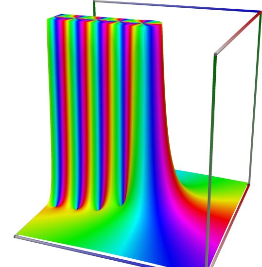

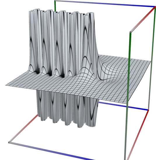
Left figure: real part of the Polygamma function, \(\psi^{(n)}(x)\). Camera angles are \(\theta=135^\circ\) and \(\phi = -12^\circ\), camera radius is -2.

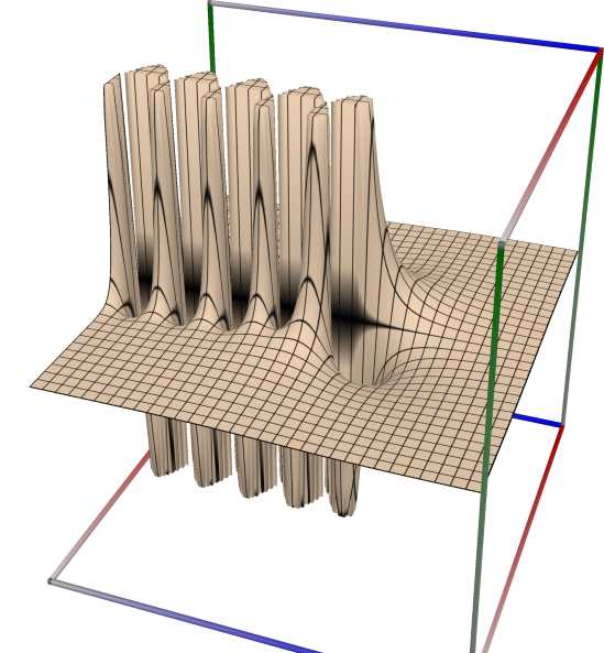
Middle figure: imaginary part of the Polygamma function, \(\psi^{(n)}(x)\). Camera angles are \(\theta=135^\circ\) and \(\phi = -12^\circ\), camera radius is -2.

Right figure: absolute value of the Polygamma function, \(\psi^{(n)}(x)\), with color-coded phase. Camera angles are \(\theta=135^\circ\) and \(\phi = -12^\circ\), camera radius is -2.

Note

This function is called psi in mpmath.

An example in Python

>>> from xlcalcnet import xreal
>>> xreal.PolyGamma(6, 7.1)
xreal('5.2359877559829887307E-1')
>>> xreal.PolyGamma(12, '4.51')
xreal('5.3518479027559984754E-1')

An example in Visual Basic

>>> from xlcalcnet import Gpr
>>> Gpr.PolyGamma(6, 7.1)
Gpr('5.2359877559829887307E-1')
>>> Gpr.PolyGamma(12, '4.51')
Gpr('5.3518479027559984754E-1')

An example with real input:

>>> from xlcalcnet import dec, mpm, gmp, fpm, apm
>>> mpm.dps = 40; m = '10'; x = '5.0'
>>> \mathrm{d}x = dec.polygamma(m, x); mx = mpm.polygamma(m, x); gx = gmp.polygamma(m, x)
>>> fx = fpm.polygamma(m, x); ax = apm.polygamma(m, x)
>>> mpm.show([\mathrm{d}x, mx, gx, fx, ax])
dec:  -8.675107579196581317296465584299728817903E-2
mpm:  -8.675107579196581317296465584299728817903e-2
gmp:  -8.675107579196581317296465584299728817903E-02
fpm:  -8.67510757919658E-02
apm:  -8.675107579196581317296465584299728817903e-2 (-8.27e-40%)

An example with complex input:

>>> from xlcalcnet import dec, mpm, gmp, fpm, apm
>>> mpm.dps = 20; m = '10'; z = '5.0 + 3j'
>>> \mathrm{d}z = dec.polygamma(m, z); mz = mpm.polygamma(m, z); gz = gmp.polygamma(m, z)
>>> fz = fpm.polygamma(m, z); az = apm.polygamma(m, z)
>>> mpm.show([\mathrm{d}z, mz, gz, fz, az],  aligned=True)
dec: -1.3604463879878727646E-2               - 8.1339079821692487285E-3j
mpm: -1.3604463879878727646e-2               - 8.1339079821692487285e-3j
gmp: -1.3604463879878727646E-02              - 8.1339079821692487285E-03j
fpm: -1.36044638798787E-02                   - 8.13390798216925E-03j
apm: -1.3604463879878727646e-2 (-4.864e-20%) - 8.1339079821692487285e-3 (-8.136e-20%)j

TriGamma function, \(\psi'(x)\)

ctx.trigamma(x)

where ctx is math53, ctxboost or ctxflint.

Returns the trigamma function \(\psi'(x), \quad x \ne 0, -1, -2, \ldots\)

The function returns the Hurwitz zeta value \(\zeta(2, x)\) if \(x\) is positive; for \(x < 0\) the polygamma reflection formula for \(n = 1\) is used to compute the result

\[\psi'(x) = \left(\frac{\pi}{\sin(\pi x)} \right)^2 - \zeta(2,1-x).\]

See also Wikipedia [1399], MathWorld [1010], NIST [25], BoostMath [137], Ehrhardt [309] (3.5.6.3).

An example in Python

>>> from xlcalcnet import xreal
>>> xreal.TriGamma(7)
xreal('5.2359877559829887307E-1')
>>> xreal.TriGamma('4.51')
xreal('5.3518479027559984754E-1')

An example in Visual Basic

>>> from xlcalcnet import Gpr
>>> Gpr.TriGamma(7)
Gpr('5.2359877559829887307E-1')
>>> Gpr.TriGamma('4.51')
Gpr('5.3518479027559984754E-1')

An example with real input:

>>> from xlcalcnet import dec, mpm, gmp, fpm, apm
>>> mpm.dps = 40; x = '5.0'
>>> \mathrm{d}x = dec.trigamma(x); mx = mpm.trigamma(x); gx = gmp.trigamma(x)
>>> fx = fpm.trigamma(x); ax = apm.trigamma(x)
>>> mpm.show([\mathrm{d}x, mx, gx, fx, ax])
dec:  2.213229557371153253613040555349140781078E-1
mpm:  2.213229557371153253613040555349140781078e-1
gmp:  2.213229557371153253613040555349140781078E-01
fpm:  2.21322955737115E-01
apm:  2.213229557371153253613040555349140781078e-1 (6.483e-40%)

An example with complex input:

>>> from xlcalcnet import dec, mpm, gmp, fpm, apm
>>> mpm.dps = 20; z = '5.0 + 3j'
>>> \mathrm{d}z = dec.trigamma(z); mz = mpm.trigamma(z); gz = gmp.trigamma(z)
>>> fz = fpm.trigamma(z); az = apm.trigamma(z)
>>> mpm.show([\mathrm{d}z, mz, gz, fz, az],  aligned=True)
dec: 1.5394122582225896863E-1              - 1.0204851974302677197E-1j
mpm: 1.5394122582225896863e-1              - 1.0204851974302677197e-1j
gmp: 1.5394122582225896863E-01             - 1.0204851974302677197E-01j
fpm: 1.53941225822259E-01                  - 1.02048519743027E-01j
apm: 1.5394122582225896863e-1 (1.376e-19%) - 1.0204851974302677197e-1 (-1.038e-19%)j

DiGamma function \(\psi(x)\)

ctx.digamma(x)

where ctx is math53, mathc53, ctxboost, ctxflint.

Returns the digamma function \(\displaystyle \psi(x) = \frac{\mathrm{d}(\log\Gamma(x)}{\mathrm{d}x} = \frac{\Gamma'(x)}{\Gamma(x)}, \quad x \ne 0, -1, -2, \ldots\).

See also Wikipedia [1381], MathWorld [990], NIST [25], BoostMath [123], Ehrhardt [309] (3.5.6.1), Ehrhardt [309] (4.2.50), Flint [805], Flint [795], Mpmath [635].

This function returns the digamma or \(\psi\) function, which is defines as

\[\psi(x) = \frac{d(\log \Gamma(x))}{\mathrm{d}x} = \frac{\Gamma'(x)}{\Gamma(x)}, \quad x \neq 0, -1, -2,\ldots\]

If \(x<0\) it is transformed to positive values with the reflection formula

\[\psi(1-x)=\psi(x) + \pi \cot(\pi x)\]

and for \(0<x<12\) the recurrence formula

\[\psi(x+1)=\psi(x) + \frac{1}{x}\]

\(\quad\) \(\quad\)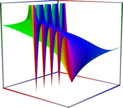

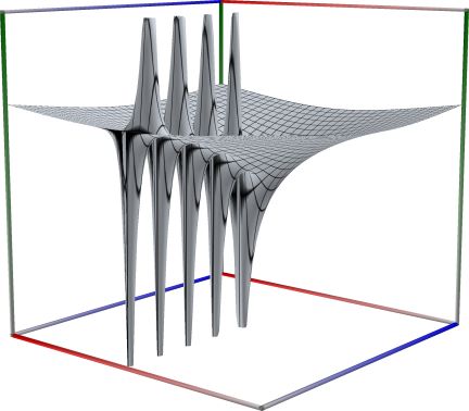
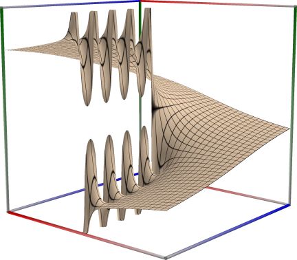
Left figure: real part of the Digamma (or psi) function \(\psi(x)\). Camera angles are \(\theta=135^\circ\) and \(\phi = -12^\circ\), camera radius is -2.

Middle figure: imaginary part of the Digamma (or psi) function \(\psi(x)\). Camera angles are \(\theta=135^\circ\) and \(\phi = -12^\circ\), camera radius is -2.

Right figure: absolute value of the Digamma (or psi) function \(\psi(x)\), with color-coded phase. Camera angles are \(\theta=135^\circ\) and \(\phi = -12^\circ\), camera radius is -2.

An example in Python

>>> from xlcalcnet import xreal
>>> xreal.Psi(7)
xreal('5.2359877559829887307E-1')
>>> xreal.Psi('4.51')
xreal('5.3518479027559984754E-1')

An example in Visual Basic

>>> from xlcalcnet import Gpr
>>> Gpr.Psi(7)
Gpr('5.2359877559829887307E-1')
>>> Gpr.Psi('4.51')
Gpr('5.3518479027559984754E-1')

An example with real input:

>>> from xlcalcnet import dec, mpm, gmp, fpm, apm
>>> mpm.dps = 40; x = '5.0'
>>> \mathrm{d}x = dec.digamma(x); mx = mpm.digamma(x); gx = gmp.digamma(x)
>>> fx = fpm.digamma(x); ax = apm.digamma(x)
>>> mpm.show([\mathrm{d}x, mx, gx, fx, ax])
dec:  1.506117668431800472726821243250930902291E+0
mpm:  1.506117668431800472726821243250930902291e+0
gmp:  1.506117668431800472726821243250930902291E+00
fpm:  1.50611766843180E+00
apm:  1.506117668431800472726821243250930902291e+0 (7.622e-40%)

An example with complex input:

>>> from xlcalcnet import dec, mpm, gmp, fpm, apm
>>> mpm.dps = 20; z = '5.0 + 3j'
>>> \mathrm{d}z = dec.digamma(z); mz = mpm.digamma(z); gz = gmp.digamma(z)
>>> fz = fpm.digamma(z); az = apm.digamma(z)
>>> mpm.show([\mathrm{d}z, mz, gz, fz, az],  aligned=True)
dec: 1.6884935312229713936E+0              + 5.8669378315167877376E-1j
mpm: 1.6884935312229713936e+0              + 5.8669378315167877376e-1j
gmp: 1.6884935312229713936E+00             + 5.8669378315167877376E-01j
fpm: 1.68849353122297E+00                  + 5.86693783151679E-01j
apm: 1.6884935312229713936e+0 (1.003e-19%) + 5.8669378315167877376e-1 (7.219e-20%)j

ctx.psi(x)

is an alias of ctx.digamma(x).

Harmonic number function, \(H_x\)

math53.harmonic(x)

Returns the Harmonic number \(H_x = \psi(x+1) + \gamma, \quad x \ne -1, -2, \ldots\).

See also: Wikipedia [1390], MathWorld [996], Ehrhardt [309] (3.6.20), Mpmath [642].

An example in Python

>>> from xlcalcnet import xreal
>>> xreal.Harmonic(10.5)
xreal('5.2359877559829887307E-1')
>>> xreal.Harmonic('10.1')
xreal('5.3518479027559984754E-1')

An example in Visual Basic

>>> from xlcalcnet import Gpr
>>> Gpr.Harmonic(10.5)
Gpr('5.2359877559829887307E-1')
>>> Gpr.Harmonic('10.1')
Gpr('5.3518479027559984754E-1')




An example with real input:

.. code-block:: pycon

    >>> from xlcalcnet import dec, mpm, gmp, fpm, apm
    >>> mpm.dps = 40; x = '1.5'
    >>> \mathrm{d}x = dec.harmonic(x); mx = mpm.harmonic(x); gx = gmp.harmonic(x)
    >>> fx = fpm.harmonic(x); ax = apm.harmonic(x)
    >>> mpm.show([\mathrm{d}x, mx, gx, fx, ax])
    dec:  1.280372305546776047832202423750313530516E+0
    mpm:  1.280372305546776047832202423750313530516e+0
    gmp:  1.280372305546776047832202423750313530516E+00
    fpm:  1.28037230554678E+00
    apm:  1.280372305546776047832202423750313530516e+0 (1.793e-39%)


An example with complex input:

.. code-block:: pycon

    >>> from xlcalcnet import dec, mpm, gmp, fpm, apm
    >>> mpm.dps = 20; z = '5.0 + 3j'
    >>> \mathrm{d}z = dec.harmonic(z); mz = mpm.harmonic(z); gz = gmp.harmonic(z)
    >>> fz = fpm.harmonic(z); az = apm.harmonic(z)
    >>> mpm.show([\mathrm{d}z, mz, gz, fz, az],  aligned=True)
    dec: 2.4127680196539160189E+0              + 4.9845848903403171494E-1j
    mpm: 2.4127680196539160189e+0              + 4.9845848903403171494e-1j
    gmp: 2.4127680196539160189E+00             + 4.9845848903403171494E-01j
    fpm: 2.41276801965392E+00                  + 4.98458489034032E-01j
    apm: 2.4127680196539160189e+0 (1.404e-19%) + 4.9845848903403171494e-1 (4.248e-20%)j