Bessel functions#
Bessel function of the 1st kind, \(J_{\nu}(x)\)#
- ctx.bessel_jv(nu, x, scaled=False)#
Returns \(J_{\nu}(x)\), the Bessel function of the 1st kind.
If scaled is True, then \(J_{\nu}(x) \cdot \exp(-|\Im(x)|)\) is returned, which means that for purely real \(x\) just \(J_{\nu}(x)\) is returned.
See also Wikipedia [1356], MathWorld [951], NIST [463], BoostMath [100], Ehrhardt [309] (3.1.3.1), Flint [822], Flint [813], Mpmath [611].
If
ctxismath53,ctxboostorctxflintreal, then \(\nu, x \in \mathbb{R}\) is exspected. Ifctxiscmath53, then \(\nu \in \mathbb{R}\) and \(x \in \mathbb{C}\) is exspected. Ifctxisctxflintcplxthen \(\nu, x \in \mathbb{C}\) is accepted.The function is defined as
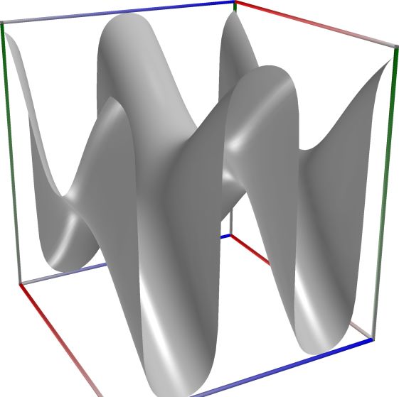
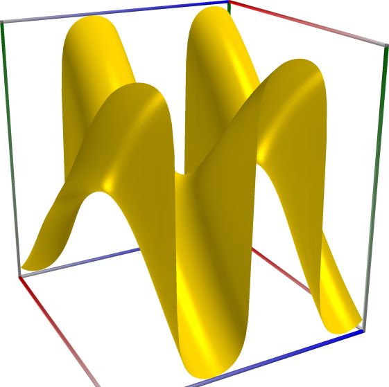
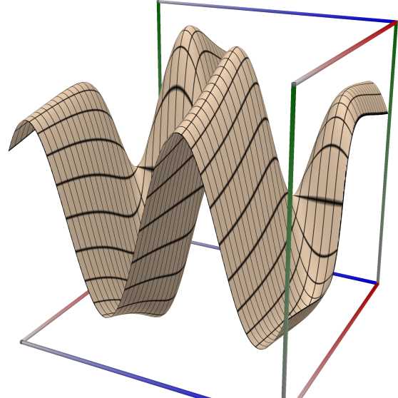
\[J_{\nu}(x) = \left(\tfrac{1}{2}x\right)^{\nu} \sum_{k=0}^\infty (-1)^k \frac{(x^2 / 4)^k}{k! \Gamma(\nu+k+1)} = \frac{1}{\Gamma(\nu+1)} \left(\frac{z}{2}\right)^{\nu} {}_0F_1\left(\nu+1, -\frac{z^2}{4}\right).\]The wpf figures below are showing the real part (left figure), imaginary part (middle figure) and absolute value with color-coded phase (right figure) of the complex function \(z = J_{\nu}(x + iy)\) with \(\nu=0\) and \(-6 \le x \le 6\) (blue axis), \(-6 \le y \le 6\) (red axis), \(-10 \le z \le 10\) (green axis). Function values are loglog-transformed.
 \(\quad\)
  \(\quad\)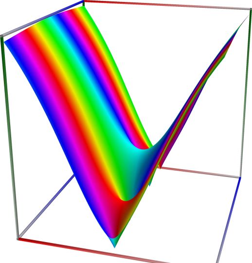
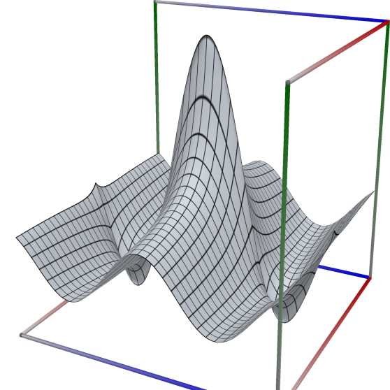
The corresponding scaled function looks like this:
 \(\quad\)
  \(\quad\)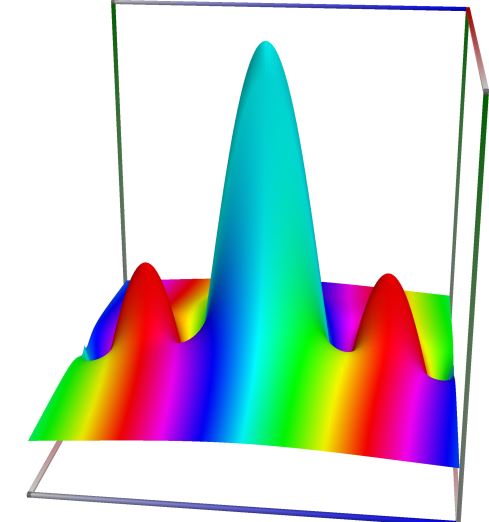
An example in Python
>>> from xlcalcnet import xreal
>>> xreal.BesselJ(3, 0.5)
xreal('5.2359877559829887307E-1')
>>> xreal.BesselJ(3, '0.51')
xreal('5.3518479027559984754E-1')
An example in Visual Basic
>>> from xlcalcnet import Gpr
>>> Gpr.BesselJ(3, 0.5)
Gpr('5.2359877559829887307E-1')
>>> Gpr.BesselJ(3, '0.51')
Gpr('5.3518479027559984754E-1')
An example with real input:
>>> from xlcalcnet import dec, mpm, gmp, fpm, apm
>>> mpm.dps = 40; n= 10; x = 30
>>> \mathrm{d}x = dec.besselj(n, x); mx = mpm.besselj(n, x); gx = gmp.besselj(n, x)
>>> fx = fpm.besselj(n, x); ax = apm.besselj(n, x)
>>> mpm.show([\mathrm{d}x, mx, gx, fx, ax])
dec:  -1.298768939985887681859474347649534305196E-1
mpm:  -1.298768939985887681859474347649534305196e-1
gmp:  -1.298768939985887681859474347649534305196E-01
fpm:  -1.29876893998589E-01
apm:  -1.298768939985887681859474347649551192015e-1 (-9.855e-30%)
An example with complex input:
>>> from xlcalcnet import dec, mpm, gmp, fpm, apm
>>> mpm.dps = 20; n= 10; z = '3 + 4j'
>>> \mathrm{d}z = dec.besselj(n, z); mz = mpm.besselj(n, z); gz = gmp.besselj(n, z)
>>> fz = fpm.besselj(n, z); az = apm.besselj(n, z)
>>> mpm.show([\mathrm{d}z, mz, gz, fz, az],  aligned=True)
dec: -2.4028734611284405858E-3               + 1.9815132418922270634E-3j
mpm: -2.4028734611284405858e-3               + 1.9815132418922270634e-3j
gmp: -2.4028734611284405858E-03              + 1.9815132418922270634E-03j
fpm: -2.40287346112844E-03                   + 1.98151324189223E-03j
apm: -2.4028734611284405858e-3 (-6.885e-20%) + 1.9815132418922270634e-3 (8.349e-20%)j
Bessel function of the 2nd kind, \(Y_{\nu}(x)\)#
- ctx.bessel_yv(nu, x, scaled=False)#
Returns \(Y_{\nu}(z)\) the Bessel function of the second kind.
If scaled is True, then \(Y_{\nu}(x) \cdot \exp(-|\Im(x)|)\) is returned, which means that for purely real \(x\) just \(Y_{\nu}(x)\) is returned.
See also Wikipedia [1357], MathWorld [952], NIST [464], BoostMath [100], Ehrhardt [309] (3.1.3.2), Flint [822], Flint [813], Mpmath [612].
If
ctxismath53,ctxboostorctxflintreal, then \(\nu, x \in \mathbb{R}\) is exspected. Ifctxiscmath53, then \(\nu \in \mathbb{R}\) and \(x \in \mathbb{C}\) is exspected. Ifctxisctxflintcplxthen \(\nu, x \in \mathbb{C}\) is accepted.The function is computed from the formula
\[Y_{\nu}(x) = \frac{\cos(\nu \pi) J_{\nu}(x) - J_{-\nu}(x)}{\sin(\nu \pi)}\]unless \(\nu = n\) is an integer in which case the limit value is computed.
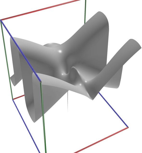
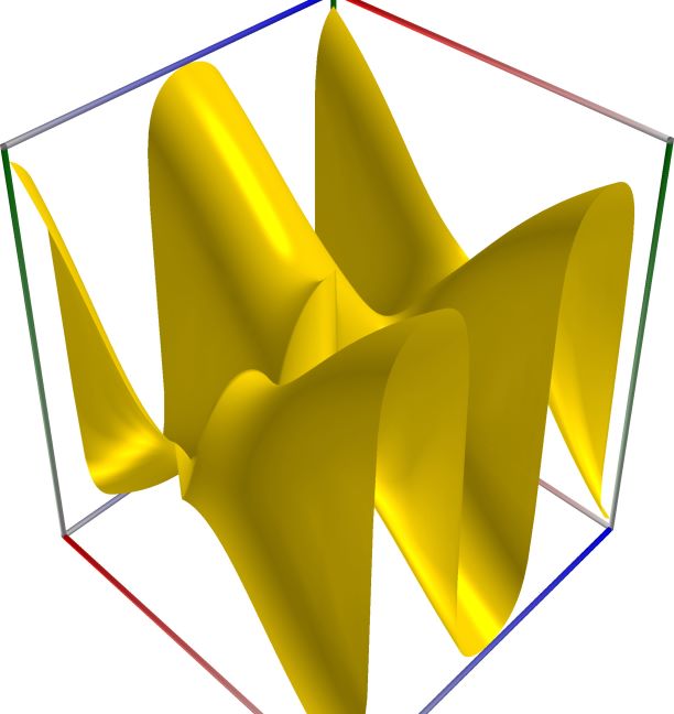
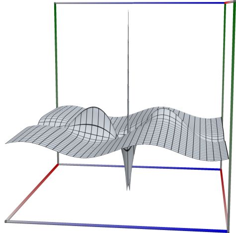
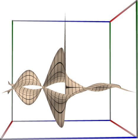
The wpf figures below are showing the real part (left figure), imaginary part (middle figure) and absolute value with color-coded phase (right figure) of the complex function \(z = Y_{\nu}(x + iy)\) with \(\nu=0\) and \(-6 \le x \le 6\) (blue axis), \(-6 \le y \le 6\) (red axis), \(-10 \le z \le 10\) (green axis). Function values are loglog-transformed.
 \(\quad\)
  \(\quad\)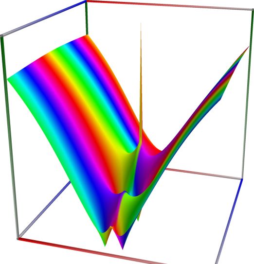
The corresponding scaled function looks like this:
 \(\quad\)
  \(\quad\)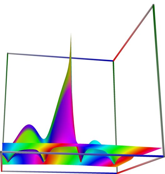
An example in Python
>>> from xlcalcnet import xreal
>>> xreal.BesselY(3, 0.5)
xreal('5.2359877559829887307E-1')
>>> xreal.BesselY(3, '0.51')
xreal('5.3518479027559984754E-1')
An example in Visual Basic
>>> from xlcalcnet import Gpr
>>> Gpr.BesselY(3, 0.5)
Gpr('5.2359877559829887307E-1')
>>> Gpr.BesselY(3, '0.51')
Gpr('5.3518479027559984754E-1')
An example with real input:
>>> from xlcalcnet import dec, mpm, gmp, fpm, apm
>>> mpm.dps = 40; n= 10; x = 30
>>> \mathrm{d}x = dec.bessely(n, x); mx = mpm.bessely(n, x); gx = gmp.bessely(n, x)
>>> fx = fpm.bessely(n, x); ax = apm.bessely(n, x)
>>> mpm.show([\mathrm{d}x, mx, gx, fx, ax])
dec:  7.505670212239711328867640811591620556875E-2
mpm:  7.505670212239711328867640811591620556875e-2
gmp:  7.505670212239711328867640811591620556875E-02
fpm:  7.50567021223971E-02
apm:  7.505670212239711328867640811591512447084e-2 (2.412e-27%)
An example with complex input:
>>> from xlcalcnet import dec, mpm, gmp, fpm, apm
>>> mpm.dps = 20; n= 10; z = '3 + 4j'
>>> \mathrm{d}z = dec.bessely(n, z); mz = mpm.bessely(n, z); gz = gmp.bessely(n, z)
>>> fz = fpm.bessely(n, z); az = apm.bessely(n, z)
>>> mpm.show([\mathrm{d}z, mz, gz, fz, az],  aligned=True)
dec: 6.7895703730606195794E+0              + 6.9959972339074326549E+0j
mpm: 6.7895703730606195794e+0              + 6.9959972339074326549e+0j
gmp: 6.7895703730606195794E+00             + 6.9959972339074326549E+00j
fpm: 6.78957037306062E+00                  + 6.99599723390743E+00j
apm: 6.7895703730606195794e+0 (3.493e-19%) + 6.9959972339074326549e+0 (3.39e-19%)j
First derivative of the Bessel function of the first kind, \(J'_{\nu}(x)\)#
- ctx.bessel_jv_prime(nu, x, scaled=False)#
Returns \(J'_{\nu}(x)\), the first derivative (with respect to \(x\)) of \(J_{\nu}(z)\), the Bessel function of the second kind.
If scaled is True, then \(J'_{\nu}(x) \cdot \exp(-|\Im(x)|)\) is returned, which means that for purely real \(x\) just \(J'_{\nu}(x)\) is returned.
See also Wikipedia [1356], MathWorld [951], NIST [463], BoostMath [100], BoostMath [122].
If
ctxismath53,ctxboostorctxflintreal, then \(\nu, x \in \mathbb{R}\) is exspected. Ifctxiscmath53, then \(\nu \in \mathbb{R}\) and \(x \in \mathbb{C}\) is exspected. Ifctxisctxflintcplxthen \(\nu, x \in \mathbb{C}\) is accepted.The function is calculated as \(J'_{\nu}(x) = \tfrac{1}{2} (J_{\nu-1}(x)- J_{\nu+1}(x))\).
An example in Python
>>> from xlcalcnet import xreal
>>> xreal.BesselJPrime(3, 0.5)
xreal('5.2359877559829887307E-1')
>>> xreal.BesselJPrime(3, '0.51')
xreal('5.3518479027559984754E-1')
An example in Visual Basic
>>> from xlcalcnet import Gpr
>>> Gpr.BesselJPrime(3, 0.5)
Gpr('5.2359877559829887307E-1')
>>> Gpr.BesselJPrime(3, '0.51')
Gpr('5.3518479027559984754E-1')
First derivative of the Bessel function of the second kind, \(Y'_{\nu}(x)\)#
- ctx.bessel_yv_prime(nu, x, scaled=False)#
Returns \(Y'_{\nu}(x)\), the first derivative (with respect to \(x\)) of \(Y_{\nu}(z)\), the Bessel function of the second kind.
If scaled is True, then \(Y'_{\nu}(x) \cdot \exp(-|\Im(x)|)\) is returned, which means that for purely real \(x\) just \(Y'_{\nu}(x)\) is returned.
See also Wikipedia [1357], MathWorld [952], NIST [464], BoostMath [100], BoostMath [122].
If
ctxismath53,ctxboostorctxflintreal, then \(\nu, x \in \mathbb{R}\) is exspected. Ifctxiscmath53, then \(\nu \in \mathbb{R}\) and \(x \in \mathbb{C}\) is exspected. Ifctxisctxflintcplxthen \(\nu, x \in \mathbb{C}\) is accepted.The function is calculated as \(Y'_{\nu}(x) = \tfrac{1}{2} (Y_{\nu-1}(x)- Y_{\nu+1}(x))\).
An example in Python
>>> from xlcalcnet import xreal
>>> xreal.BesselYPrime(3, 0.5)
xreal('5.2359877559829887307E-1')
>>> xreal.BesselYPrime(3, '0.51')
xreal('5.3518479027559984754E-1')
An example in Visual Basic
>>> from xlcalcnet import Gpr
>>> Gpr.BesselYPrime(3, 0.5)
Gpr('5.2359877559829887307E-1')
>>> Gpr.BesselYPrime(3, '0.51')
Gpr('5.3518479027559984754E-1')
Boost: Zeros \(j_{\nu, m}\) of the Bessel function of the first kind: \(J_{\nu}(j_{\nu, m})=0\)#
- ctx.bessel_jv_zero(nu, m)#
where
ctxismath53orctxboost.For a real order \(\nu \ge 0\) and a positive integer \(m\), returns \(j_{\nu, m}\), the \(m\)-th positive zero of the Bessel function of the first kind \(J_{\nu}(x)\).
See also Wikipedia [1356], MathWorld [1022], NIST [465], BoostMath [125], Mpmath [671].
An example in Python
>>> from xlcalcnet import xreal
>>> xreal.BesselJZero(3, 0.5)
xreal('5.2359877559829887307E-1')
>>> xreal.BesselJZero(3, '0.51')
xreal('5.3518479027559984754E-1')
An example in Visual Basic
>>> from xlcalcnet import Gpr
>>> Gpr.BesselJZero(3, 0.5)
Gpr('5.2359877559829887307E-1')
>>> Gpr.BesselJZero(3, '0.51')
Gpr('5.3518479027559984754E-1')
Boost: Zeros \(y_{\nu, m}\) of the Bessel function of the first kind: \(Y_{\nu}(y_{\nu, m})=0\)#
- ctx.bessel_yv_zero(nu, m)#
where
ctxismath53orctxboost.For a real order \(\nu \ge 0\) and a positive integer \(m\), returns \(y_{\nu, m}\), the \(m\)-th positive zero of the Bessel function of the second kind \(Y_{\nu}(x)\).
See also Wikipedia [1357], MathWorld [1023], NIST [465], BoostMath [125], Mpmath [672].
An example in Python
>>> from xlcalcnet import xreal
>>> xreal.BesselJZero(3, 0.5)
xreal('5.2359877559829887307E-1')
>>> xreal.BesselJZero(3, '0.51')
xreal('5.3518479027559984754E-1')
An example in Visual Basic
>>> from xlcalcnet import Gpr
>>> Gpr.BesselJZero(3, 0.5)
Gpr('5.2359877559829887307E-1')
>>> Gpr.BesselJZero(3, '0.51')
Gpr('5.3518479027559984754E-1')