Ctrl+K

XlCalcNet Documentation

  • Preface

Getting started

  • Setup and general usage
    • Setting up XlCalcNet
    • General and user interface functions
    • Calling Python from C#
    • Using XlCalcNet with spreadsheet formulas
    • Mathematical functions based on Mpmath, Gmpy2 and Python-Flint (only Python)
    • Mathematical functions in fixed precision
    • Mathematical functions based on XlCalcNet2
    • A quick look at Numpy
    • A quick look at Matplotlib and related libraries
    • A quick look at Pandas and Xlxswriter
    • A quick look at Scipy
    • A quick look at R, RStudio and Rpy2
  • Basic floating point functions
    • Operator overloading, general real functions
    • Machine constants, general
    • Properties of numbers
    • Integer related functions
    • Floating point functions for real numbers
    • Fraction and remainder related functions
    • Functions related to mantissa width and exponent range
    • Mathematical Constants
  • Elementary scalar functions (real and complex)
    • Complex components
    • Roots and quadratic, cubic, and quartic equations
    • Exponential and related functions
    • Logarithms and related functions
    • Power functions
    • Trigonometric functions, in radians
    • Trigonometric functions, in multiples of \(\pi\)
    • Hyperbolic functions
    • Inverse trigonometric functions, in radians
    • Inverse hyperbolic functions
    • Factorials, Gamma and related functions
    • Miscellaneous functions
  • Statistical Distributions
    • Introduction to random variables and distributions
    • Base class for univariate distributions
    • Base class for continuous univariate distributions
    • Base class for discrete univariate distributions
    • Closed form distributions, based on elementary functions
      • Boost: Arcsine Distribution
      • Boost: Cauchy distribution
      • Boost: Exponential distribution
      • Boost: Gumbel (Generalized Extreme Value distribution Type-I) distribution
      • Boost: Hyperexponential Distribution
      • !!!Boost: Kumaraswamy distribution
      • Boost: Laplace distribution
      • Boost: Logistic distribution
      • Boost: Pareto distribution
      • Boost: Rayleigh distribution
      • Boost: Triangular Distribution
      • Boost: Uniform distribution
      • Boost: Weibull (Minimum-Type-III) distribution
      • Dagum (Burr Type III) distribution
      • Fisk (log-logistic) distribution
      • Fréchet (Maximum/Minimum-Type-II or Inverse Weibull) distribution
      • Generalized Extreme Value (Maximum) or GEV distribution
      • Generalized Pareto distribution
      • Gompertz-Makeham distribution
      • Lomax distribution
      • Shifted Gompertz distribution
      • Singh-Maddala (Burr Type XII) distribution
    • Closed form distributions, based on the error function
      • !!!Boost: Lévy distribution
      • Boost: Lognormal (Johnson \(S_L\)) distribution
      • !!!Boost: Moyal Distribution
      • Boost: Normal (Johnson \(S_N\)) distribution
      • Boost: Skew normal Distribution
      • Boost: Wald (or Inverse Gaussian) distribution
      • Birnbaum-Saunders Distribution
      • Exponentially Modified Gaussian (EMG) distribution
      • Folded normal distribution
      • Half-normal distribution
      • Johnson \(S_B\) distribution
      • Johnson \(S_U\) distribution
      • Normal maximum distribution, \(\rho_{ij, i \ne j} = 0\)
      • Normal maximum modulus distribution, \(\rho_{ij, i \ne j} = 0\)
      • Sinh-arcsinh normal distribution
      • Truncated normal distribution
    • Closed form distributions, based on the incomplete gamma function
      • !!!Boost: Chi Distribution
      • Boost: Chi-Squared distribution
      • Boost: Gamma (Pearson Type III, Erlang) distribution
      • Boost: Inverse chisquared distribution
      • Boost: Inverse Gamma (Pearson Type V) distribution
      • !!!Boost: Maxwell Distribution
      • !!!Boost: Nakagami distribution
      • Amoroso distribution
      • Distribution of the logarithm of a \(\chi^2\) random variable
      • Hypoexponential (Generalized Erlang) Distribution
      • Lindley distribution (generalized)
      • Skew exponential power distribution
      • Stacy (generalized gamma) distribution
    • Closed form distributions, based on the incomplete beta function
      • Boost: Beta (Pearson Type I and II) distribution
      • Boost: Central Fisher F distribution
      • Boost: Student \(t\) (Pearson Type VII) distribution
      • Distribution of the negative logarithm of a beta variable
      • Beta-prime (Pearson Type VI) distribution
      • Generalized Beta (Type 1) distribution
      • Generalized Beta (Type 2) distribution
      • Generalized logistic distribution (JKB Types I - IV)
      • Generalized beta-exponential distribution
      • Feller-Pareto distribution
      • Fisher \(z\) distribution
      • Skew t-distribution (Jones)
      • Pearson’s rho distribution (under \(H_0\))
    • Noncentral distributions
      • Boost: Noncentral \(\chi^2\) distribution
      • Boost: Noncentral Student \(t\) distribution
      • Boost: Noncentral Fisher \(F\) distribution
      • Boost: Noncentral Beta Type I distribution
      • Noncentral Chi distribution
      • Rice (Nakagami-n) distribution
      • Noncentral distribution of the sample correlation coefficient
      • Distribution of the logarithm of a noncentral Beta Type II variable
      • Noncentral distribution (Type I) of Fisher’s \(R^2\)
      • Distribution of the logarithm of a noncentral Fisher \(1-R^2\) variable
      • Doubly non-central Student \(t\) distribution
      • Doubly non-central Fisher \(F\) distribution
    • Distributions related to multiple comparisons of means
      • Overview and literature
      • Normal maximum distribution, \(\rho_{ij, i \ne j} = \rho\)
      • Normal maximum modulus distribution, \(\rho_{ij, i \ne j} = \rho\)
      • Normal maximum distribution, \(\rho_{ij, i \ne j} = \lambda_i \lambda_j\)
      • Normal maximum modulus distribution, \(\rho_{ij, i \ne j} = \lambda_i \lambda_j\)
      • Normal range distribution
      • Studentized maximum distribution
      • Studentized maximum modulus distribution
      • Distribution of Dunnett’s \(t\), one-sided
      • Distribution of Dunnett’s \(t\), two-sided
      • Nair’s \(t\)-distribution
      • Halperin’s \(t\)-distribution
      • Nelson’s \(h\)-distribution
      • Studentized range distribution
    • Distributions related to multivariate statistical analysis
      • Distribution of the sum of the negative logarithms of independent beta variables
      • Distribution of the product of independent beta variables
      • Distribution of Wilks’ \(\Lambda\)
      • Distribution of Wilks’ \(L_{vc}\)
      • Distribution of Wilks’ \(L_{vcm}\)
      • Distribution of Wilks’ test of independence of \(p\) variates
      • Distribution of Wilks’ test of independence of \(k\) groups of variates
      • Distribution of Mauchly’s test of sphericity vs general structure
      • Distribution of Box’s test of equality of covariance matrices, equal sample sizes
      • Distribution of Box’s test of equality of k covariance matrices, unequal sample sizes
      • Distribution of Box’s test for same multivariate normal distributions, unequal sample sizes
      • Distribution of the modified likelihood ratio test (LRT) for a given covariance matrix
      • Distribution of the modified likelihood ratio test (LRT) for a given covariance matrix and mean vector
      • Central distribution of Roy’s largest root
      • Central distribution of Pillai’s \(V\)
      • Central distribution of Hotelling’s \(T^2\)
      • Noncentral Distribution of Wilks’ \(\Lambda\): MANOVA
      • Noncentral Distribution of Wilks’ \(\Lambda\): Canonical Correlation
    • Miscellaneous continuous distributions
      • Boost: Kolmogorov-Smirnov distribution (limiting form)
      • Boost: Landau Distribution
      • Boost: Holtsmark distribution
      • Boost: Map-Airy distribution
      • Boost: Saspoint5 distribution
      • Lévy alpha-stable distribution
      • Pearson Type IV distribution
      • Meixner distribution
      • Voigt Profile Distribution
      • Wrapped Cauchy distribution
      • Wrapped normal distribution
      • Von Mises distribution
      • Generalized inverse Gaussian distribution
      • Harmonic distribution
      • Halphen A distribution
      • Halphen B distribution
      • Halphen IB distribution
      • Generalized hyperbolic distribution
      • Hyperbolic distribution
      • Variance-gamma distribution
    • Elementary discrete (lattice) distributions
      • Boost: Bernoulli distribution
      • Boost: Geometric distribution
      • Boost: Poisson distribution
      • Boost: Binomial distribution
      • Boost: Negative binomial distribution
      • Boost: Classical hypergeometric distribution
      • Log-series distribution
      • Zeta distribution
      • Skellam distribution
      • Delaporte distribution
      • Beta-Poisson distribution (Quinkert)
      • Beta-binomial distribution
      • Beta-negative binomial distribution (Waring)
      • Negative hypergeometric distribution
      • Pólya-Eggenberger distribution
      • General hypergeometric distribution
      • Noncentral hypergeometric distribution, Fisher alternatives
    • Discrete (lattice) distributions related to (stratified) rank tests
      • Wilcoxon signed rank T distribution, continuous data
      • Noncentral Wilcoxon signed rank T distribution, Bennett alternatives
      • Mann-Whitney U distribution, continuous data
      • Noncentral Mann-Whitney U distribution, Lehmann alternatives
      • Noncentral Mann-Whitney U distribution, Milton alternatives
      • Kendall’s tau distribution, continuous data
      • Jonckheere-Terpsta \(T\) distribution, continuous data
      • Generalized Page \(L\) distribution, continuous data
      • Noncentral generalized Page \(L\) distribution, Milton alternatives
    • Discrete (non-lattice) distributions related to rank tests
      • Cochran-Friedman-Quade distribution
      • Kruskal-Wallis distribution
  • Numerical calculus
    • Introduction
    • DAMath: Numerical Rootfinding and Minimization
    • Boost/Math: Root Finding and Minimization Algorithms
    • Mpmath: Rootfinding and optimization
    • DAMath: Numerical Quadrature
    • Boost/Math: Numerical integration
    • Mpmath: Numerical integration
    • Mpmath: Numerical inverse Laplace transform
    • Boost/Odeint: Ordinary differential equations
    • Mpmath: Numerical differentiation
    • Mpmath: Asymptotic expansions
    • Mpmath: Function approximation
    • Mpmath: Sums, products, limits and extrapolation
    • Mpmath: Number identification
    • Mpmath: Polynomials
    • Eigen: Polynomials
    • Eigen/MinPack: non linear optimization
    • Eigen/CppOptLib: multidimensional optimization
    • Flint/Functions for polynomials
    • Flint/Power series and Taylor arithmetic
    • Flint/Verified numerical differentiation
    • Flint/Verified numerical integration
  • Eigen: Dense and Sparse Matrices
    • Creating scalars and matrices
    • Read-only properties: information about a matrix
    • Accessing and setting parts of a matrix
    • Changing the shape of a matrix and/or the order of coefficients
    • Basic arithmetic operations
    • Descriptive Statistics
    • Standard decompositions and linear solving
    • Singular Value and Eigen (selfadjoint) decompositions
    • Eigen decompositions of general square matrices
    • Eigen: Functions of matrix argument
    • Eigen: Fast Fourier Transform
  • Numpy: use with multiprecision data types
    • Numpy array creation from shape or value
    • Numpy array creation from existing data
    • Building special arrays for numerical work
    • Numpy indexing
    • Numpy basic array manipulation routines
    • Numpy array manipulation: Transpose-like operations
    • Numpy array manipulation: Changing number of dimensions
    • Numpy array manipulation: Joining arrays
    • Numpy array manipulation: Splitting and tiling arrays
    • Numpy array manipulation: Adding and removing elements
    • Numpy array manipulation: Rearranging elements
    • Numpy array manipulation: Sorting
    • Numpy array manipulation: Searching
    • Numpy mathematical functions: Sums, products, differences
    • Numpy mathematical functions: Extrema Finding
    • Numpy mathematical functions: Arithmetic operations, elementwise
    • Numpy mathematical functions: Averages and variances
    • Numpy mathematical functions: Matrix and vector products
    • Numpy logical functions: Truth value testing
    • Numpy mathematical functions: Integer and fractional
    • Numpy mathematical functions: Miscellaneous
    • Summary and examples: Numpy utility functions
    • Arithmetic operations with scalars and iterables
    • Numerical transformations and descriptive statistics
    • Standard decompositions and linear solving
    • Singular Value and Eigen decompositions
    • Analytic functions of a matrix
    • Discrete Fourier transform (DFT)
    • Flint/Functions for matrices

Special Functions

  • Elliptic functions and related
    • Carlson symmetric elliptic integrals
    • Legendre elliptic integrals (elliptic parameter \(m\))
    • Legendre elliptic integrals (elliptic modulus \(k\)), and related functions
    • Jacobi elliptic functions
    • Jacobi theta functions and related functions
    • Conversions of parameters of Weierstrass \(\wp\)
    • Weierstrass elliptic functions, in terms of elliptic period ratio \(\tau\)
    • Modular forms, in terms of half-period \(\omega_1\) and elliptic period ratio \(\tau\)
  • Lerch’s phi and related
    • Lerch’s transcendent and Lerch’s zeta
    • Polygamma and related functions
    • Polylogarithm and related functions
    • Hurwitz zeta and related functions
    • Riemann zeta function, and related functions
  • Hypergeometric function \(\,_0F_1\) and related
    • Hypergeometric Limit Function \(\,_0F_1\)
    • Bessel functions
    • Modified Bessel functions
    • Spherical Bessel functions
    • Modified spherical Bessel functions
    • Hankel functions
    • Airy functions
    • Kelvin functions
  • Hypergeometric function \(\,_1F_1\) and related
    • Hypergeometric Functions \(\,_1F_1\) (Kummer) and \(U\) (Tricomi)
    • Incomplete gamma functions
    • Coulomb, Whittaker and parabolic cylinder function
    • Error function and related functions
    • Exponential integrals, and related functions
  • Hypergeometric functions \(\,_2F_1\) and \(\,_1F_2\) (and related functions)
    • Gauss Hypergeometric Function \(\,_2F_1\)
    • Chebyshev, Gegenbauer and Jacobi polynomials
    • Legendre polynomials and related
    • Incomplete beta functions
    • Hypergeometric function \({}_1F_2\)
    • Scorer functions
    • Struve functions
    • Anger, Weber and Lommel functions

Supporting Functions

  • Algebra with random variables
    • Probability density function (pdf)
    • Probability mass function (pmf)
    • Cumulative distribution function (cdf)
    • Quantile function
    • Characteristic function
    • Moment generating function
    • Cumulant generating function
    • Probability generating function
    • Factorial Moments
    • Raw Moments
    • Central Moments
    • Cumulants
  • Series and integrals
    • Finite series algorithms for selected distributions
    • Infinite series algorithms for selected functions and distributions
    • Finite series for lattice distributions, based on factorial moments
    • Efficient integration of bell-shaped functions
    • Verified numerical integration
  • Pmf vectors
    • Basic discrete (lattice) distribution functions
    • Discrete (lattice) distribution functions related to (stratified) rank tests
    • Discrete (non-lattice) distribution functions related to rank tests
  • Fast approximations
    • Approximations based on the normal distribution
    • Approximations based on the chi-squared distribution
    • Approximations based on the central \(t\), \(F\) or beta distribution
    • Approximations based on the noncentral chi-squared distribution
    • Approximations based on the noncentral F or beta distribution
    • Approximations based on hypergeometric functions of scalar argument

Gallery of Plots

  • Visualisation of datasets
    • Bar Charts
    • Line and lollipop charts
    • Area Plots
    • Boxplot, Violinplot and Raincloud plot
    • Correlation and regression
    • Financial plots (requires mplfinance)
    • Geographic data (requires cartopy)
    • Geographic data (requires geopandas)
    • Parts of a whole
    • Arcplots, dendrograms, heatmaps and clustermaps
    • PlotTable
    • Flow and connections
    • Circular plots and flows
    • Network data (requires networkx)
  • Visualisation of functions and curves (2D)
    • Introduction to 2D functions and curves
    • Basic curves
    • Spirals
    • Decorative curves
    • General curve families
    • Field lines
    • Contours
    • Complex functions rendered as contours
    • Streams, barbs and quivers (some require cartopy)
  • Bitmaps
    • Fractals: introduction
    • Fractals related to the Mandelbrot set
    • Fractals related to the Julia set
    • Newton Fractals
    • Domain coloring options
    • Domain coloring: Examples part 1
  • Matplotlib 3D Graphics
    • Introduction
    • Matplotlib: 3D Graphics, part 2
    • S3dlib: Basic geometric figures
    • S3dlib: Real functions
    • S3dlib: Parametric Surfaces
    • S3dlib: Image mapping and clipping
    • S3dlib: Edge-to-edge surface coloring
    • S3dlib: Decorative parametric surfaces
    • S3dlib: Geometric and color datagrid mapping (requires scipy)
    • S3dlib: Implicit surfaces (requires scikit-image)
  • Plotly
    • General surface plots in 3D
    • Geographical plots
    • Sankey plots

Interactive 3D Wpf Plots

  • Wpf: Altitude surfaces in 3D, real and complex functions
    • Special techniques for height surfaces, real and complex functions
    • Scatterplots and building 3D scenes
    • Height plots of general bivariate real functions
  • Wpf: Parametric surfaces
    • Surfaces of translation
    • Surfaces of revolution: spheres and related
    • Generalisations of common surfaces
    • Minimal surfaces
    • Nonorientable (one-sided) Surfaces
    • Decorative parametric surfaces
  • Wpf: Path surfaces in 3D
    • Introduction to path surfaces
    • Functions with real input and complex results
    • Characteristic functions of statistical distributions
    • Helices and related curves traced on cylinders, cones and spheres
    • Coil springs
    • General knots
    • Torus knots
    • Lissajous knots
    • Polynomial knots
  • Wpf: Built-in 3D objects
    • Builtin solids with support for textures
    • Builtin solids without support for textures
    • Platonic solids, and related solids

User library: numerical

  • Additional Classes
    • User defined functions based on multiple precision arithmetic (Python)
    • User defined functions based on fixed precision arithmetic (C#)
    • User defined functions based on arbitrary precision arithmetic (C#)
    • Scalar functions
  • Distribution functions
    • Distributions related to multiple comparisons of means
    • Discrete (lattice) distribution functions related to (stratified) rank tests
    • Discrete (non-lattice) distribution functions related to rank tests
  • Inferential statistics
    • Basic classical statistical tests (stratified)
    • Basic classical statistical tests for 2 independent samples (stratified)
    • Basic classical statistical tests for 2 correlated samples (stratified)
    • Analysis of variance (ANOVA), orthogonal polynomials, and analysis of means (AOM)
    • Multiple comparisons of means
    • Nonparametric statistical tests, 1 or 2 samples
    • Nonparametric statistical tests, k samples
    • Multivariate statistical tests
  • Addditional elementary functions (real arguments, double precision)
    • Additional root, exponential, logarithmic and power functions
    • Additional Trigonometric functions (real arguments only)
    • Additional real error functions (real arguments only)
    • Additional real gamma functions (real arguments only)
    • Additional real incomplete gamma functions (real arguments only)
  • Addditional special functions (real arguments, double precision)
    • Conversions of parameters of elliptic functions
    • Additional elliptic integrals
    • Bulirsch elliptic integrals
    • Maple style elliptic integrals
    • Jacobi theta functions at \(x=0\) for \(0 \le q <1\)
    • Inverse Jacobi elliptic functions
    • Lemniscate functions
    • Neville theta functions
    • Polygamma, and related functions
    • Polylogarithm, and related functions
    • Riemann zeta, and related functions
    • Bessel functions of integer order
    • Modified Bessel functions of integer order
    • Integrals of zero-order Bessel functions
    • Kelvin functions of order 0
    • Synchrotron functions
    • Error function, and related functions
    • Exponential integrals, and related functions
    • Coulomb, Whittaker and parabolic cylinder function
    • Hypergeometric pFq, and related functions
    • Miscellaneous functions
  • Addditional special functions (complex arguments, double precision)
    • Conversions of parameters of Weierstrass \(\wp\)
    • Weierstrass elliptic functions, in terms of (real) lattice invariants \(g_2, g_3\)
    • Weierstrass elliptic functions, in terms of (real) lattice roots \(e_1, e_2\)
    • Weierstrass elliptic functions, in terms of lattice half-periods \(\omega_1\) and \(\omega_2\)
  • Addditional special functions (Mpmath)
    • Mpmath: Conversions of parameters of elliptic functions
    • Related to Lerch’s phi
    • Additional numbertheoretic functions
    • Generalized hypergeometric functions
    • Appell Functions
    • Q Functions
    • Further generalizations of gamma and hypergeometric functions

Back matter

  • License and History
    • Mozilla Public License Version 2.0
    • History

Indices

  • General Index
  • .rst

Helices and related curves traced on cylinders, cones and spheres

Contents

  • Cylindrical helix
  • Conical helix based on Archimedes spiral (spiral of Pappus)
  • Conical helix based on Fermat’s spiral
  • Conical helix based on the logarithmic spiral (Concho-Spiral)
  • Conical helix based on the hyperbolic spiral
  • Rhumb line of the sphere
  • Clelia
  • Spherical helix
  • Satellite curve
  • Seiffert’s spiral

Helices and related curves traced on cylinders, cones and spheres#

See also: https://en.wikipedia.org/wiki/Helix

See also: https://mathworld.wolfram.com/Helix.html

See also: https://mathcurve.com/courbes3d.gb/helice/helice.shtml

The helices are the curves the tangents of which form a constant angle a with respect to a fixed plane (P0), or a fixed direction d (orthogonal to (P0)). Therefore, the notion of helix in mathematics is more connected to a mountain road with constant slope than to the helix of a boat!

Examples (note that the helices are described by their base or the surface on which they are traced):
  • the straight line (lines on a surface are therefore helices of this surface)

  • the cylindrical helix (base = circle)

  • the conical helix (traced on a vertical cone of revolution, base = logarithmic spiral)

  • the elliptic helix (base = ellipse)

  • the spherical helix (traced on a sphere, base = epicycloid)

  • the helix of the paraboloid (base = involute of a circle).

  • the helix of the one-sheeted hyperboloid (traced on the one-sheeted hyperboloid)

  • the striction line of the milk carton

NOTE: the item “H. Stop of y, v [STOP2]” determines the diameter of the helix.

Cylindrical helix#

See also: https://mathcurve.com/courbes3d.gb/helicecirculaire/helicecirculaire.shtml

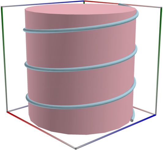
The cylindrical helix can be defined as a helix traced on a vertical cylinder of revolution, or a rhumb line of this cylinder (i.e., in both cases, a curve forming a constant angle with respect to the axis of the cylinder), or a geodesic of this cylinder (in other words, a curve that becomes a line when the cylinder is developed) or a solenoid with linear bore. Intrinsic characterization: constant curvature and torsion.

The radius of the helix is a, and its shift is (it is the distance between two consecutive coils) and b is sometimes called reduced shift of the helix. The angle of the helix is the constant angle (equal to ) formed by its tangent with respect to any plane orthogonal to Oz. The helix is right-handed when e = 1 (it “goes up” counterclockwise and an observer located outside of it sees it going up from left to right) and left-handed when e = - 1 (it “goes up” clockwise).

An example in C#

double a = 0.2;
// double b = 1.0;
double b = 0.2;
var x = a * Math.Cos(t);
var y = a * Math.Sin(t);
var z = b * t;

Some text
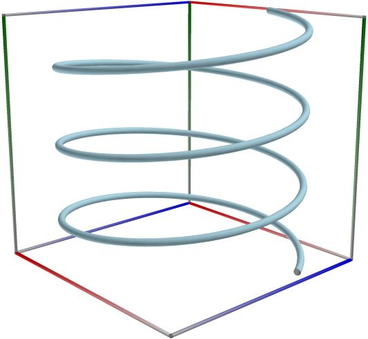
Path_SpiralCylindrical_a \(\quad\) PathD_SpiralCylindrical_a

Left figure: Cylindrical helix. Perspective camera. Camera angles are \(\theta=90^\circ\) and \(\phi = 90^\circ\).

Right figure: Cylindrical helix. Perspective camera. Camera angles are \(\theta=90^\circ\) and \(\phi = 180^\circ\).

Conical helix based on Archimedes spiral (spiral of Pappus)#

See also: https://en.wikipedia.org/wiki/Conical_spiral

See also: https://mathworld.wolfram.com/ConicalSpiral.html

See also: https://mathcurve.com/courbes3d.gb/helicecirculaire/helicecirculaire.shtml

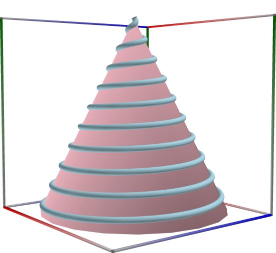
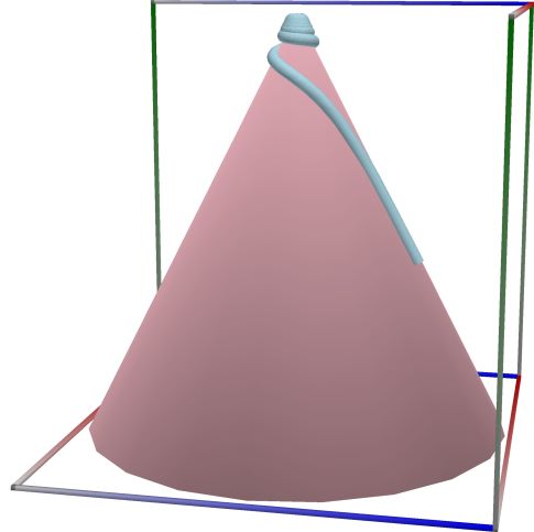
The conical helix can be defined as a helix traced on a cone of revolution (i.e. a curve forming a constant angle with respect to the axis of the cone), or a rhumb line of this cone (i.e. a curve forming a constant angle with the meridians); it is not a geodesic of the cone. In concrete terms, we get a conical helix when we trace a path with constant slope on a cone placed vertically.

The projection on xOy is a logarithmic spiral (), which is also the locus of the intersection between the tangents and xOy; the curve obtained by developing the cone is also a logarithmic spiral. As for all helices, it is a geodesic of the vertical cylinder based on the aforementioned spiral, projection of the curve on xOy. The principal normal is always perpendicular to Oy. The radii of curvature and torsion are proportional to z. The helix is right-handed when (it “goes up” clockwise) and left-handed when (it “goes up” counterclockwise).

An example in C#

double a = 1.0;
double phi = t * Math.PI;
double rphi = a * phi;
var x = (rphi * Math.Cos(phi));
var y = (rphi * Math.Sin(phi));
//var z = (0.2 * t);
var z = (1.2 * t);

Some text
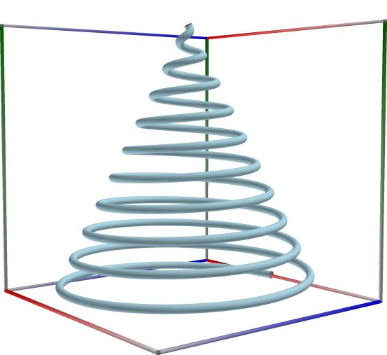
Path_SpiralAConical_a \(\quad\) PathD_SpiralAConical_a

Left figure: Conical helix based on Archimedes spiral. Perspective camera. Camera angles are \(\theta=90^\circ\) and \(\phi = 90^\circ\).

Right figure: Conical helix based on Archimedes spiral. Perspective camera. Camera angles are \(\theta=90^\circ\) and \(\phi = 180^\circ\).

Conical helix based on Fermat’s spiral#

See also: https://en.wikipedia.org/wiki/Conical_spiral

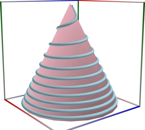
Conical helix based on Fermat’s spiral

An example in C#

double a = 1.0;
double m = 0.2 / Math.PI;
double phi = t * Math.PI;
double rphi = a * Math.Sqrt(phi);
var x = (rphi * Math.Cos(phi));
var y = (rphi * Math.Sin(phi));
var z = (m * rphi);

Some text
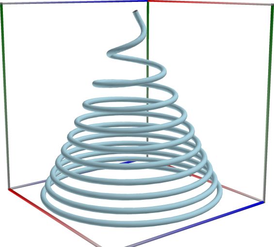
Path_SpiralFConical_a \(\quad\) PathD_SpiralFConical_a

Left figure: Conical helix based on Fermat’s spiral. Perspective camera. Camera angles are \(\theta=90^\circ\) and \(\phi = 90^\circ\).

Right figure: Conical helix based on Fermat’s spiral. Perspective camera. Camera angles are \(\theta=90^\circ\) and \(\phi = 180^\circ\).

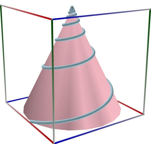
Conical helix based on the logarithmic spiral (Concho-Spiral)#

See also: https://mathworld.wolfram.com/Concho-Spiral.html

See also: https://en.wikipedia.org/wiki/Conchospiral

An example in C#

double k = 0.1;
double a = 1.0;
double m = 0.2 / Math.PI;
double phi = t * Math.PI;
double rphi = a * Math.Exp(k * phi);
var x = (rphi * Math.Cos(phi));
var y = (rphi * Math.Sin(phi));
var z = (m * rphi);

Some text
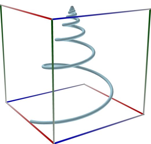
Path_SpiralLConical_a \(\quad\) PathD_SpiralLConical_a

Left figure: Conical helix based on the logarithmic spiral. Perspective camera. Camera angles are \(\theta=90^\circ\) and \(\phi = 90^\circ\).

Right figure: Conical helix based on the logarithmic spiral. Perspective camera. Camera angles are \(\theta=90^\circ\) and \(\phi = 180^\circ\).

Conical helix based on the hyperbolic spiral#

See also: https://mathcurve.com/courbes3d.gb/spiralehyperbolique/spiralehyperbolique.shtml

The hyperbolic conical spirals are the spirals traced on a cone of revolution that can be projected on the plane perpendicular to the axis onto a hyperbolic spiral with center the vertex of the cone.

An example in C#

double a = 1.0;
double m = 0.2 / Math.PI;
double phi = t * Math.PI;
double rphi = a / Math.Sqrt(phi);
var x = (rphi * Math.Cos(phi));
var y = (rphi * Math.Sin(phi));
var z = (m * rphi);

Some text
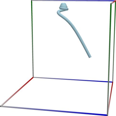
Path_SpiralHConical_a \(\quad\) PathD_SpiralHConical_a

Left figure: Conical helix based on the hyperbolic spiral. Perspective camera. Camera angles are \(\theta=90^\circ\) and \(\phi = 90^\circ\).

Right figure: Conical helix based on the hyperbolic spiral. Perspective camera. Camera angles are \(\theta=90^\circ\) and \(\phi = 180^\circ\).

Rhumb line of the sphere#

See also: https://mathcurve.com/courbes3d.gb/loxodromie/sphereloxodromie.shtml

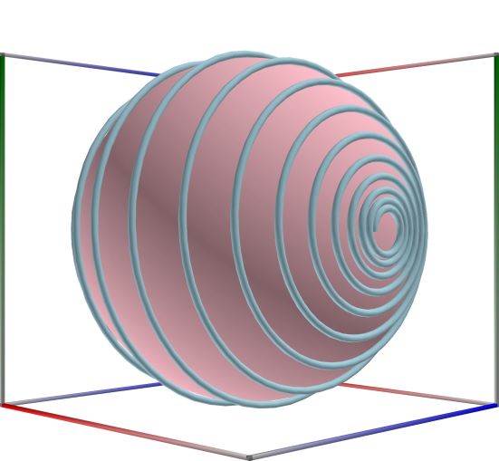
The rhumb lines of the sphere, associated to a given axis, are the curves that form a constant angle with the parallel (or the meridians). Do not mistake the rhumb lines for the spherical helices, that form a constant angle with the equatorial plane, nor for the clelias.

The rhumb lines correspond to the straight lines in Mercator coordinates ; in other words, on the maps of the Earth that use the Mercator projection, the rhumb lines are represented by straight lines. The angle a that the images of the rhumb lines form on the map with respect to the horizontal is the same as the angle they form on the sphere with respect to the parallels. If we know the geographic coordinates and of two points, the angle a associated to the shortest rhumb line joining these two points is obtained by the formula: and the length is given by: . The notion of rhumb line is opposed to that of geodesic, shortest path joining two points on the sphere, which is an arc of a great circle

An example in C#

double R = 1.0;
double alpha = 0.05;
double k = Math.Tan(alpha);
var x = R * Math.Cos(t) / Math.Cosh(k * t);
var y = R * Math.Sin(t) / Math.Cosh(k * t);
var z = R * Math.Tanh(k * t);

Some text
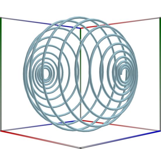
Path_SphericalRhumbline_a \(\quad\) PathD_SphericalRhumbline_a

Left figure: Rhumb line of the sphere. Perspective camera. Camera angles are \(\theta=90^\circ\) and \(\phi = 90^\circ\).

Right figure: Rhumb line of the sphere. Perspective camera. Camera angles are \(\theta=90^\circ\) and \(\phi = 180^\circ\).

Clelia#

See also: https://mathcurve.com/courbes3d.gb/clelie/clelie.shtml

See also: https://en.wikipedia.org/wiki/Cl%C3%A9lie

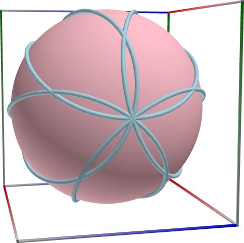
The clelias are the loci of a point M on a meridian of a sphere rotating at constant speed w around the polar axis, the point M also moving at constant speed nw along this meridian. Therefore, physically, we obtain a clelia when peeling an orange or when rewinding regularly a spherical wool ball.

When n is rational with numerator p and denominator q:

In this case, the curve is composed of 2p patterns, obtained from the base pattern by rotations of axis Oz and angles \(2k \pi / n\) and \(p + 2k \pi / n\) .

When p and q are odd, the curve is composed of p patterns, obtained from the base pattern by rotations of axis Oz and angles \(2k \pi / n\) .

An example in C#

double R = 1.0;
double n1 = 5.0 / 2.0;    // Example 1
var x = R * Math.Cos(n1 * t) * Math.Cos(t);
var y = R * Math.Cos(n1 * t) * Math.Sin(t);
var z = R * Math.Sin(n1 * t);

Some text
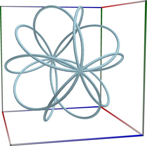
Path_SphericalClelia_a \(\quad\) PathD_SphericalClelia_a

Left figure: Clelia. Perspective camera. Camera angles are \(\theta=90^\circ\) and \(\phi = 90^\circ\).

Right figure: Clelia. Perspective camera. Camera angles are \(\theta=90^\circ\) and \(\phi = 180^\circ\).

Spherical helix#

See also: https://mathworld.wolfram.com/SphericalSpiral.html

See also: https://mathworld.wolfram.com/SphericalHelix.html

See also: https://mathcurve.com/courbes3d.gb/helicespheric/helicespheric.shtml

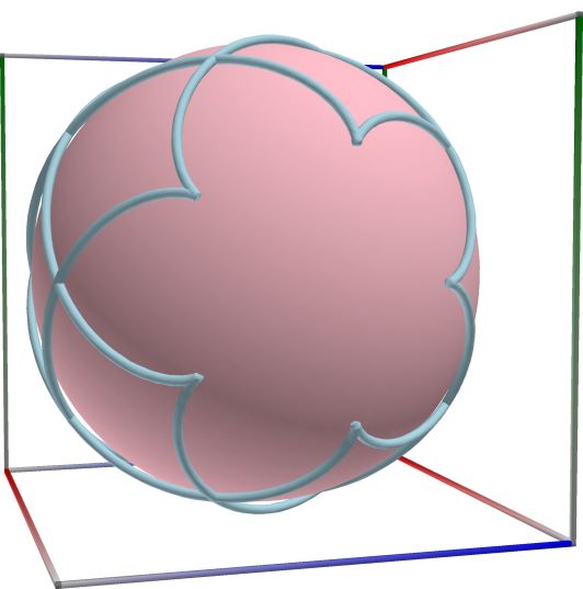
A spherical cycloid is the locus of a point on a circle rolling without slipping on a fixed circle, the angle between the two circles remaining constant equal to ; here, a is the radius of the fixed circle, that of the moving circle, and xOy the plane where lies the fixed circle.

When = 0, we get the hypocycloid, and when = , the epicycloid; apart from these two cases, the cycloid is traced on the sphere corresponding to both the base and the rolling circles, hence its name of spherical cycloid. The center W of this sphere is the point on Oz at height and its radius is . Therefore, the spherical cycloid is a roulette of the motion of a sphere over a sphere.

An example in C#

double q = 5.0 / 2.0;    // Example 1
//double q = 2.0 / 5.0;    // Example 2
//double q = 1.0 / 5.0;    // Example 3
double R = 1.0;
double k = q / (q + 2);
var x = R * (k * Math.Cos(t) * Math.Cos(k * t) + Math.Sin(t) * Math.Sin(k * t));
var y = R * (k * Math.Sin(t) * Math.Cos(k * t) - Math.Cos(t) * Math.Sin(k * t));
var z = R * Math.Sqrt(1 - k * k) * Math.Cos(k * t);

Some text
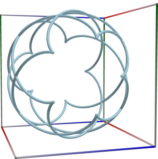
Path_SphericalHelix_a \(\quad\) PathD_SphericalHelix_a

Left figure: Spherical helix. Perspective camera. Camera angles are \(\theta=90^\circ\) and \(\phi = 90^\circ\).

Right figure: Spherical helix. Perspective camera. Camera angles are \(\theta=90^\circ\) and \(\phi = 180^\circ\).

Satellite curve#

See also: https://mathcurve.com/courbes3d.gb/satellite/satellite.shtml

See also: https://mathcurve.com/courbes3d.gb/capareda/capareda.shtml

The satellite curves are the various trajectories of a point M on a given great circle of a sphere rotating around one of its axes, while M has a uniform motion along the circle. These curves can also be seen as the trajectories of points on a circle in uniform rotation around an axis, this axis being itself in uniform rotation around an axis passing by the center of the circle.

The name of satellite curve comes from the fact that the trajectory, in the frame associated to the Earth, of a satellite in uniform circular rotation around the center of the Earth is such a curve: see for example this book (pages 177 to 181).

In the above parametrization, the sphere centered on O turns around Oz and the plane of the circle forms an angle with respect to xOy; k is the ratio of the speed of rotation of M on the circle over the speed of rotation of the sphere around its axis.

Special cases of satellite curves include:
  • the clelias when the great circle meets the axis of rotation of the sphere ().

  • the spherical helices when (in the second definition above, the circle rolls without slipping on a fixed circle); it is the case where the curve has cuspidal points.

An example in C#

double R = 1.0;
//double alpha = 1 * Math.PI / 2;  // This corresponds to clelias
double alpha = 3 * Math.PI / 4;
double k = 3.0 / 4.0;
//double k = -Math.Cos(alpha);  // This corresponds to spherical helices
var x = R * (Math.Cos(alpha) * Math.Cos(t) * Math.Cos(k * t) - Math.Sin(t) * Math.Sin(k * t));
var y = R * (Math.Cos(alpha) * Math.Sin(t) * Math.Cos(k * t) + Math.Cos(t) * Math.Sin(k * t));
var z = R * Math.Sin(alpha) * Math.Cos(k * t);

Some text
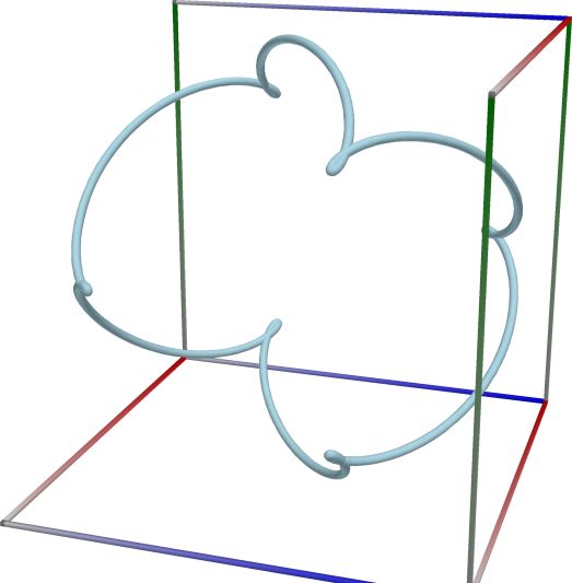
Path_SphericalSatellite_a \(\quad\) PathD_SphericalSatellite_a

Left figure: Satellite curve. Perspective camera. Camera angles are \(\theta=90^\circ\) and \(\phi = 90^\circ\).

Right figure: Satellite curve. Perspective camera. Camera angles are \(\theta=90^\circ\) and \(\phi = 180^\circ\).

Seiffert’s spiral#

See also: https://en.wikipedia.org/wiki/Seiffert%27s_spiral

See also: https://mathworld.wolfram.com/SeiffertsSphericalSpiral.html

See also: https://en.wikipedia.org/wiki/Cylindrical_coordinate_system

The spherical curve obtained when moving along the surface of a sphere with constant speed, while maintaining a constant angular velocity with respect to a fixed diameter (Erdős 2000). This curve is given in cylindrical coordinates by the parametric equations

\[r = sn(s,k),\]
\[\theta = k s,\]
\[z=cn(s,k),\]

where k is a positive constant and sn(s) and cn(s) are Jacobi elliptic functions (Whittaker and Watson 1990, pp. 527-528).

Erdős (2000) provides a derivation of the equations of this curve, as well as an analysis of its properties, including conditions for obtaining periodic orbits.

Erdős, P. “Spiraling the Earth with C. G. J. Jacobi.” Amer. J. Phys. 68, 888-895, 2000.

Seiffert. “Über eine neue geometrische Einführung in die Theorie der elliptischen Funktionen.” Wissensch. Beiträge Jahresber. Städtischen Realschule zu Charlottenburg, Ostern. 1896.

Whittaker, E. T. and Watson, G. N. A Course in Modern Analysis, 4th ed. Cambridge, England: Cambridge University Press, 1990.

previous

Characteristic functions of statistical distributions

next

Coil springs

Contents
  • Cylindrical helix
  • Conical helix based on Archimedes spiral (spiral of Pappus)
  • Conical helix based on Fermat’s spiral
  • Conical helix based on the logarithmic spiral (Concho-Spiral)
  • Conical helix based on the hyperbolic spiral
  • Rhumb line of the sphere
  • Clelia
  • Spherical helix
  • Satellite curve
  • Seiffert’s spiral

By Dietrich Hadler

© Copyright 2026, Dietrich Hadler. .

Last updated on Aug 19, 2026.