Hypergeometric Functions \(\,_1F_1\) (Kummer) and \(U\) (Tricomi)#
Kummer’s Confluent Hypergeometric Function \({}_1F_1(a,b;x)\)#
- ctx.hyperg_1f1(a, b, x)#
Returns \(\displaystyle {}_1F_1(a,b;x)\), the confluent hypergeometric function of the first kind, where \(b \ne 0,-1,-2,\ldots\).
See also Wikipedia [1361], MathWorld [972], NIST [200], BoostMath [109], Ehrhardt [309] (3.8.3), Abramowitz and Stegun. [2], Flint [823], Flint [816], Mpmath [619].
Here \(a, b\) and \(x\) are, in general, complex numbers. However, if
ctxismath53, then \(a,b \in \mathbb{R}\) and \(x \in \mathbb{R}\) is exspected. Ifctxiscmath53, then \(a, b \in \mathbb{R}\) and \(x \in \mathbb{C}\) is exspected. Ifctxisctxflintthen \(a, b, x \in \mathbb{C}\) is accepted.The function is defined as \(\displaystyle {}_1F_1(a,b;x) = \sum_{k=0}^\infty\frac{(a)_k}{(b)_k} \frac{z^k}{k!}\).
 \(\quad\)
  \(\quad\)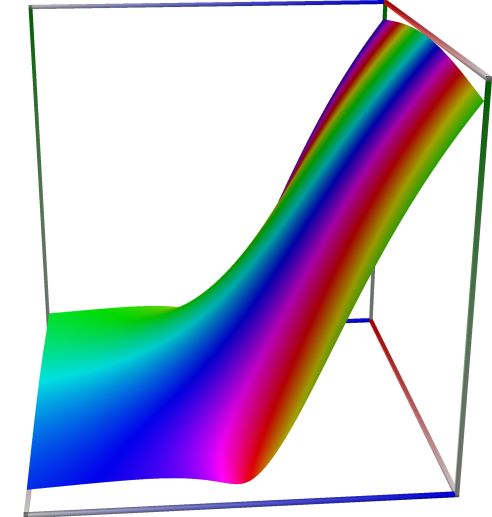
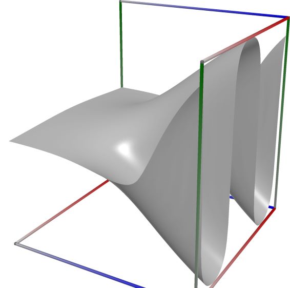
Left figure: real part of Kummer’s Confluent Hypergeometric Function \({}_1F_1(a,b;x)\). Camera angles are \(\theta=135^\circ\) and \(\phi = -12^\circ\), camera radius is -2.
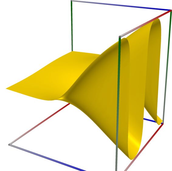
Middle figure: imaginary part of Kummer’s Confluent Hypergeometric Function \({}_1F_1(a,b;x)\). Camera angles are \(\theta=135^\circ\) and \(\phi = -12^\circ\), camera radius is -2.
Right figure: absolute value of Kummer’s Confluent Hypergeometric Function \({}_1F_1(a,b;x)\), with color-coded phase. Camera angles are \(\theta=135^\circ\) and \(\phi = -12^\circ\), camera radius is -2.
An example in Python
>>> from xlcalcnet import xreal
>>> xreal.Hyperg1F1(4,5,0.5)
xreal('5.2359877559829887307E-1')
>>> xreal.Hyperg1F1(14,15,0.5)
xreal('5.3518479027559984754E-1')
An example in Visual Basic
>>> from xlcalcnet import Gpr
>>> Gpr.Hyperg1F1(4,5,0.5)
Gpr('5.2359877559829887307E-1')
>>> Gpr.Hyperg1F1(14,15,0.5)
Gpr('5.3518479027559984754E-1')
An example with real input:
>>> from xlcalcnet import dec, mpm, gmp, fpm, apm
>>> mpm.dps = 40; a = 11.0; b = 12.0; x = 3.0
>>> \mathrm{d}x = dec.hyp1f1(a, b, x); mx = mpm.hyp1f1(a, b, x); gx = gmp.hyp1f1(a, b, x)
>>> fx = fpm.hyp1f1(a, b, x); ax = apm.hyp1f1(a, b, x)
>>> mpm.show([\mathrm{d}x, mx, gx, fx, ax])
dec:  1.601638079764459102142699167478416306125E+1
mpm:  1.601638079764459102142699167478416306125e+1
gmp:  1.601638079764459102142699167478416306125E+01
fpm:  1.60163807976446E+01
apm:  1.601638079764459102142699167478416306125e+1 (1.147e-39%)
An example with complex input:
>>> from xlcalcnet import dec, mpm, gmp, fpm, apm
>>> mpm.dps = 20; a = '11.0 + 2.0j'; b = '12.0 + 3.0j'; z = '3.0 + 4.0j'
>>> \mathrm{d}z = dec.hyp1f1(a, b, z); mz = mpm.hyp1f1(a, b, z); gz = gmp.hyp1f1(a, b, z)
>>> fz = fpm.hyp1f1(a, b, z); az = apm.hyp1f1(a, b, z)
>>> mpm.show([\mathrm{d}z, mz, gz, fz, az], aligned=True)
dec: -1.7071475892855456616E+1               - 6.5250702392280765696E+0j
mpm: -1.7071475892855456616e+1               - 6.5250702392280765696e+0j
gmp: -1.7071475892855456616E+01              - 6.5250702392280765696E+00j
fpm: -1.70714758928555E+01                   - 6.52507023922808E+00j
apm: -1.7071475892855456616e+1 (-1.588e-19%) - 6.5250702392280765696e+0 (-5.192e-20%)j
Regularized Kummer Confluent Hypergeometric Function, \({}_1\widetilde{F}_1(a,b;x)\)#
- ctx.hyperg_1f1r(a, b, x)#
Returns \(\displaystyle {}_1\widetilde{F}_1(a,b;z)\), the regularized Kummer confluent hypergeometric function.
See also Wikipedia [1361], MathWorld [268], NIST [200], BoostMath [109], Ehrhardt [309] (3.8.4), Abramowitz and Stegun. [2], Flint [823], Flint [816], Mpmath [619].
Here \(a, b\) and \(x\) are, in general, complex numbers. However, if
ctxismath53, then \(a,b \in \mathbb{R}\) and \(x \in \mathbb{R}\) is exspected. Ifctxiscmath53, then \(a, b \in \mathbb{R}\) and \(x \in \mathbb{C}\) is exspected. Ifctxisctxflintthen \(a, b, x \in \mathbb{C}\) is accepted.We have \(\displaystyle {}_1\widetilde{F}_1(a,b;z) = \frac{1}{\Gamma(b)} {}_1F_1(a;b;z) = \mathbf{M}(a,b;x) = \frac{1}{\Gamma(b)} M(a;b;z)\), for \(b \ne 0, -1, -2, \cdots\).
If \(b = 0, -1, -2, \cdots = -n\), the corresponding limit \(\displaystyle {}_1\widetilde{F}_1(a,b;x) = \frac{(a)_{n+1}}{(n+1)!} x^{n+1} {}_1F_1(a+n+1,n+2;x)\) is calculated.
An example in Python
>>> from xlcalcnet import xreal
>>> xreal.Hyperg1F1r(4,5,0.5)
xreal('5.2359877559829887307E-1')
>>> xreal.Hyperg1F1r(14,15,0.5)
xreal('5.3518479027559984754E-1')
An example in Visual Basic
>>> from xlcalcnet import Gpr
>>> Gpr.Hyperg1F1r(4,5,0.5)
Gpr('5.2359877559829887307E-1')
>>> Gpr.Hyperg1F1r(14,15,0.5)
Gpr('5.3518479027559984754E-1')
An example with real input:
>>> from xlcalcnet import dec, mpm, gmp, fpm, apm
>>> mpm.dps = 40; a = 11.0; b = 12.0; x = 3.0
>>> \mathrm{d}x = dec.hyp1f1r(a, b, x); mx = mpm.hyp1f1r(a, b, x); gx = gmp.hyp1f1r(a, b, x)
>>> fx = fpm.hyp1f1r(a, b, x); ax = apm.hyp1f1r(a, b, x)
>>> mpm.show([\mathrm{d}x, mx, gx, fx, ax])
dec:  4.012441076850997830844905321765312615552E-7
mpm:  4.012441076850997830844905321765312615552e-7
gmp:  4.012441076850997830844905321765312615552E-07
fpm:  4.01244107685100E-07
apm:  4.012441076850997830844905321765312615552e-7 (2.728e-39%)
An example with complex input:
>>> from xlcalcnet import dec, mpm, gmp, fpm, apm
>>> mpm.dps = 20; a = '11.0 + 2.0j'; b = '12.0 + 3.0j'; z = '3.0 + 4.0j'
>>> \mathrm{d}z = dec.hyp1f1r(a, b, z); mz = mpm.hyp1f1r(a, b, z); gz = gmp.hyp1f1r(a, b, z)
>>> fz = fpm.hyp1f1r(a, b, z); az = apm.hyp1f1r(a, b, z)
>>> mpm.show([\mathrm{d}z, mz, gz, fz, az], aligned=True)
dec: -5.0984734340262287981E-7               + 4.4090124699188539207E-7j
mpm: -5.0984734340262287981e-7               + 4.4090124699188539207e-7j
gmp: -5.0984734340262287981E-07              + 4.4090124699188539207E-07j
fpm: -5.09847343402623E-07                   + 4.40901246991885E-07j
apm: -5.0984734340262287982e-7 (-7.922e-20%) + 4.4090124699188539207e-7 (9.161e-20%)j
Tricomi’s Confluent Hypergeometric Function, \(U(a,b;x)\)#
- ctx.hyperg_u(a, b, x)#
Returns Tricomi’s confluent hypergeometric function of the second kind, \(\displaystyle U(a,b;x)\).
See also Wikipedia [1361], MathWorld [973], NIST [200], Ehrhardt [309] (3.8.5), Flint [823], Flint [816], Mpmath [621].
Here \(a, b\) and \(x\) are, in general, complex numbers. However, if
ctxismath53, then \(a,b \in \mathbb{R}\) and \(x \in \mathbb{R}\) is exspected. Ifctxiscmath53, then \(a, b \in \mathbb{R}\) and \(x \in \mathbb{C}\) is exspected. Ifctxisctxflintthen \(a, b, x \in \mathbb{C}\) is accepted.For all \(z \ne 0\) and \(b \notin \mathbb{Z}\) (but valid for all \(b\) as a limit) we have
\[U(a,b;x) = \frac{\Gamma(1-b)}{\Gamma(1+a-b)} M(a,b;c;z) + \frac{\Gamma(1-b)}{\Gamma(a)} x^{1-b} M(1+a-b,2-b;x)\]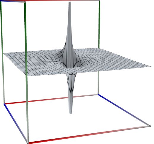 \(\quad\)
  \(\quad\)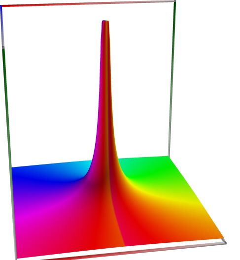
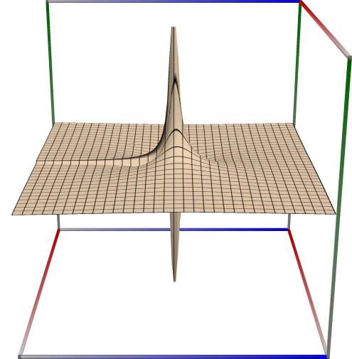
Left figure: real part of Tricomi’s Confluent Hypergeometric Function, \(U(a,b;x)\). Camera angles are \(\theta=135^\circ\) and \(\phi = -12^\circ\), camera radius is -2.
Middle figure: imaginary part of Tricomi’s Confluent Hypergeometric Function, \(U(a,b;x)\). Camera angles are \(\theta=135^\circ\) and \(\phi = -12^\circ\), camera radius is -2.
Right figure: absolute value of Tricomi’s Confluent Hypergeometric Function, \(U(a,b;x)\), with color-coded phase. Camera angles are \(\theta=135^\circ\) and \(\phi = -12^\circ\), camera radius is -2.
An example in Python
>>> from xlcalcnet import xreal
>>> xreal.HypergU(4,5.1,0.5)
xreal('5.2359877559829887307E-1')
>>> xreal.HypergU(14,15.2,0.5)
xreal('5.3518479027559984754E-1')
An example in Visual Basic
>>> from xlcalcnet import Gpr
>>> Gpr.HypergU(4,5.1,0.5)
Gpr('5.2359877559829887307E-1')
>>> Gpr.HypergU(14,15.2,0.5)
Gpr('5.3518479027559984754E-1')
An example with real input:
>>> from xlcalcnet import dec, mpm, gmp, fpm, apm
>>> mpm.dps = 40; a = 11.0; b = 12.0; x = 3.0
>>> \mathrm{d}x = dec.hyperu(a, b, x); mx = mpm.hyperu(a, b, x); gx = gmp.hyperu(a, b, x)
>>> fx = fpm.hyperu(a, b, x); ax = apm.hyperu(a, b, x)
>>> mpm.show([\mathrm{d}x, mx, gx, fx, ax])
dec:  5.645029269476762237012198908251339283194E-6
mpm:  5.645029269476762237012198908251339283194e-6
gmp:  5.645029269476762237012198908251339283194E-06
fpm:  5.64502926947676E-06
apm:  5.645029269476762237012198908251339283194e-6 (7.757e-40%)
An example with complex input:
>>> from xlcalcnet import dec, mpm, gmp, fpm, apm
>>> mpm.dps = 20; a = '11.0 + 2.0j'; b = '12.0 + 3.0j'; z = '3.0 + 4.0j'
>>> \mathrm{d}z = dec.hyperu(a, b, z); mz = mpm.hyperu(a, b, z); gz = gmp.hyperu(a, b, z)
>>> fz = fpm.hyperu(a, b, z); az = apm.hyperu(a, b, z)
>>> mpm.show([\mathrm{d}z, mz, gz, fz, az], aligned=True)
dec: 2.0656756869642262785E-7              + 5.4116585242285070055E-8j
mpm: 2.0656756869642262785e-7              + 5.4116585242285070055e-8j
gmp: 2.0656756869642262785E-07             + 5.4116585242285070055E-08j
fpm: 2.06567568696423E-07                  + 5.41165852422851E-08j
apm: 2.0656756869642262785e-7 (9.776e-20%) + 5.4116585242285070055e-8 (4.665e-20%)j
Generalized Laguerre polynomials, \(L^{(a)}_n (x)\)#
- ctx.laguerre_l(n, a, x)#
where
ctxismath53orctxflint.Note: math53.laguerre(z, n, alpha)
Returns \(\displaystyle L^{(a)}_n (x) = \binom{n+a}{n} M(-n,a+1,x) = \frac{\Gamma(n+a+1)}{\Gamma(n+1)\Gamma(a+1)} {}_1F_1(-n,a+1,x)\), the generalized Laguerre polynomials of degree \(n \geq 0\) with parameter \(a; x \geq 0\) and \(a > -1\) are the standard ranges.
For integer degree \(n \ge 0\) and integer order \(m \ge 0\), we have, as a special case, the (associated) Laguerre polynomial \(L_n^m(x) = L_n^{(m)}(x)\). If \(m = 0\), it is just called Laguerre polynomial: \(L_n(x) = L_n^0(x) = L_n^{(0)}(x)\)
These polynomials are orthogonal on the interval \((0,\infty)\), with respect to the weight function \(w(x) = e^{-x}x^a\). The following standard recurrence formulas are used:
\begin{eqnarray} L^{(a)}_0 (x) & = & 1 \\ L^{(a)}_1 (x) & = & -x+1+a \nonumber \\ nL^{(a)}_n (x)& = & (2n+a-1-x) L^{(a)}_{n-1}(x) - (n+a-1) L^{(a)}_{n-2}(x). \nonumber \end{eqnarray}See also Wikipedia [1419], MathWorld [1000], NIST [419], BoostMath [130], Ehrhardt [309] (3.7.10) and (3.7.12), Flint [825], Flint [821], Mpmath [665].
An example in Python
>>> from xlcalcnet import xreal
>>> xreal.Laguerre(2, 3, 2, 0.5)
xreal('5.2359877559829887307E-1')
>>> xreal.Laguerre('6, 2, 0.51')
xreal('5.3518479027559984754E-1')
An example in Visual Basic
>>> from xlcalcnet import Gpr
>>> Gpr.Laguerre(2, 3, 2, 0.5)
Gpr('5.2359877559829887307E-1')
>>> Gpr.Laguerre('6, 2, 0.51')
Gpr('5.3518479027559984754E-1')
Hermite polynomial (physicist), \(H_n(x)\)#
- ctx.hermite_h(n, z)#
Returns \(\displaystyle H_n(z)\), the Hermite polynomial (physicist) of degree \(n\).
See also Wikipedia [1413], MathWorld [997], NIST [419], BoostMath [127], Ehrhardt [309] (3.7.7) and (3.8.11.4), Ehrhardt [309] Flint [825], Flint [821], Mpmath [662].
Here \(n\) and \(x\) are, in general, complex numbers. However, if
ctxismath53, then \(n \in \mathbb{R}\) and \(x \in \mathbb{R}\) is exspected. Ifctxiscmath53, then \(n \in \mathbb{R}\) and \(x \in \mathbb{C}\) is exspected. Ifctxisctxflintthen \(n, x \in \mathbb{C}\) is accepted.We have \(\displaystyle H_n(z) = 2^n \sqrt{\pi} \left( \frac{1}{\Gamma\left(\frac{1-n}{2}\right)} \,_1F_1\left(-\frac{n}{2}, \frac{1}{2}, z^2\right) - \frac{2z}{\Gamma\left(-\frac{n}{2}\right)} \,_1F_1\left(\frac{1-n}{2}, \frac{3}{2}, z^2\right) \right)\), where \(\displaystyle \frac{1}{\Gamma\left(n \right)}\) is evaluated calling the reciprocal gamma function.
For integer \(n \ge 0\), the \(H_n\) are orthogonal on the interval \((-\infty, \infty)\), with respect to the weight function \(w(x) = e^{-x^2}\). They can be computed with the standard recurrence formulas:
\begin{eqnarray} H_0 (x) & = & 1 \\ H_1 (x) & = & 2x \nonumber \\ H_n (x)& = & 2x H_{n-1}(x) - 2(n-1) H_{n-2}(x). \nonumber \end{eqnarray}An example in Python
>>> from xlcalcnet import xreal
>>> xreal.HermiteH(2, 0.5)
xreal('5.2359877559829887307E-1')
>>> xreal.HermiteH(6, 0.51)
xreal('5.3518479027559984754E-1')
An example in Visual Basic
>>> from xlcalcnet import Gpr
>>> Gpr.HermiteH(2, 0.5)
Gpr('5.2359877559829887307E-1')
>>> Gpr.HermiteH(6, 0.51)
Gpr('5.3518479027559984754E-1')
Hermite polynomials (probabilist) \(\operatorname{He}_n(x)\)#
- math53.hermite_he(n, x)#
Returns \(\operatorname{He}_n(x) = 2^{-n/2} H_n(x/\sqrt{2})\), the probabilist’s Hermite polynomial of degree \(n \ge 0\).
For integer \(n\), the \(\operatorname{He}_n\) are orthogonal on the interval \((-\infty, \infty)\), with respect to the weight function \(w(x) = \exp(-x^2/2)\). They are computed with the standard recurrence formulas:
\begin{eqnarray} \operatorname{He}_0 (x) & = & 1 \\ \operatorname{He}_1 (x) & = & x \nonumber \\ \operatorname{He}_n (x)& = & x \operatorname{He}_{n-1}(x) - (n-1) \operatorname{He}_{n-2}(x). \nonumber \end{eqnarray}See also Wikipedia [1413], MathWorld [997], NIST [419], BoostMath [127], Ehrhardt [309] (3.7.8), Flint [825], Flint [821], Mpmath [662].
An example in Python
>>> from xlcalcnet import xreal
>>> xreal.HermiteHe(2, 0.5)
xreal('5.2359877559829887307E-1')
>>> xreal.HermiteHe(6, 0.51)
xreal('5.3518479027559984754E-1')
An example in Visual Basic
>>> from xlcalcnet import Gpr
>>> Gpr.HermiteHe(2, 0.5)
Gpr('5.2359877559829887307E-1')
>>> Gpr.HermiteHe(6, 0.51)
Gpr('5.3518479027559984754E-1')