Ctrl+K

XlCalcNet Documentation

  • Preface

Getting started

  • Setup and general usage
    • Setting up XlCalcNet
    • General and user interface functions
    • Calling Python from C#
    • Using XlCalcNet with spreadsheet formulas
    • Mathematical functions based on Mpmath, Gmpy2 and Python-Flint (only Python)
    • Mathematical functions in fixed precision
    • Mathematical functions based on XlCalcNet2
    • A quick look at Numpy
    • A quick look at Matplotlib and related libraries
    • A quick look at Pandas and Xlxswriter
    • A quick look at Scipy
    • A quick look at R, RStudio and Rpy2
  • Basic floating point functions
    • Operator overloading, general real functions
    • Machine constants, general
    • Properties of numbers
    • Integer related functions
    • Floating point functions for real numbers
    • Fraction and remainder related functions
    • Functions related to mantissa width and exponent range
    • Mathematical Constants
  • Elementary scalar functions (real and complex)
    • Complex components
    • Roots and quadratic, cubic, and quartic equations
    • Exponential and related functions
    • Logarithms and related functions
    • Power functions
    • Trigonometric functions, in radians
    • Trigonometric functions, in multiples of \(\pi\)
    • Hyperbolic functions
    • Inverse trigonometric functions, in radians
    • Inverse hyperbolic functions
    • Factorials, Gamma and related functions
    • Miscellaneous functions
  • Statistical Distributions
    • Introduction to random variables and distributions
    • Base class for univariate distributions
    • Base class for continuous univariate distributions
    • Base class for discrete univariate distributions
    • Closed form distributions, based on elementary functions
      • Boost: Arcsine Distribution
      • Boost: Cauchy distribution
      • Boost: Exponential distribution
      • Boost: Gumbel (Generalized Extreme Value distribution Type-I) distribution
      • Boost: Hyperexponential Distribution
      • !!!Boost: Kumaraswamy distribution
      • Boost: Laplace distribution
      • Boost: Logistic distribution
      • Boost: Pareto distribution
      • Boost: Rayleigh distribution
      • Boost: Triangular Distribution
      • Boost: Uniform distribution
      • Boost: Weibull (Minimum-Type-III) distribution
      • Dagum (Burr Type III) distribution
      • Fisk (log-logistic) distribution
      • Fréchet (Maximum/Minimum-Type-II or Inverse Weibull) distribution
      • Generalized Extreme Value (Maximum) or GEV distribution
      • Generalized Pareto distribution
      • Gompertz-Makeham distribution
      • Lomax distribution
      • Shifted Gompertz distribution
      • Singh-Maddala (Burr Type XII) distribution
    • Closed form distributions, based on the error function
      • !!!Boost: Lévy distribution
      • Boost: Lognormal (Johnson \(S_L\)) distribution
      • !!!Boost: Moyal Distribution
      • Boost: Normal (Johnson \(S_N\)) distribution
      • Boost: Skew normal Distribution
      • Boost: Wald (or Inverse Gaussian) distribution
      • Birnbaum-Saunders Distribution
      • Exponentially Modified Gaussian (EMG) distribution
      • Folded normal distribution
      • Half-normal distribution
      • Johnson \(S_B\) distribution
      • Johnson \(S_U\) distribution
      • Normal maximum distribution, \(\rho_{ij, i \ne j} = 0\)
      • Normal maximum modulus distribution, \(\rho_{ij, i \ne j} = 0\)
      • Sinh-arcsinh normal distribution
      • Truncated normal distribution
    • Closed form distributions, based on the incomplete gamma function
      • !!!Boost: Chi Distribution
      • Boost: Chi-Squared distribution
      • Boost: Gamma (Pearson Type III, Erlang) distribution
      • Boost: Inverse chisquared distribution
      • Boost: Inverse Gamma (Pearson Type V) distribution
      • !!!Boost: Maxwell Distribution
      • !!!Boost: Nakagami distribution
      • Amoroso distribution
      • Distribution of the logarithm of a \(\chi^2\) random variable
      • Hypoexponential (Generalized Erlang) Distribution
      • Lindley distribution (generalized)
      • Skew exponential power distribution
      • Stacy (generalized gamma) distribution
    • Closed form distributions, based on the incomplete beta function
      • Boost: Beta (Pearson Type I and II) distribution
      • Boost: Central Fisher F distribution
      • Boost: Student \(t\) (Pearson Type VII) distribution
      • Distribution of the negative logarithm of a beta variable
      • Beta-prime (Pearson Type VI) distribution
      • Generalized Beta (Type 1) distribution
      • Generalized Beta (Type 2) distribution
      • Generalized logistic distribution (JKB Types I - IV)
      • Generalized beta-exponential distribution
      • Feller-Pareto distribution
      • Fisher \(z\) distribution
      • Skew t-distribution (Jones)
      • Pearson’s rho distribution (under \(H_0\))
    • Noncentral distributions
      • Boost: Noncentral \(\chi^2\) distribution
      • Boost: Noncentral Student \(t\) distribution
      • Boost: Noncentral Fisher \(F\) distribution
      • Boost: Noncentral Beta Type I distribution
      • Noncentral Chi distribution
      • Rice (Nakagami-n) distribution
      • Noncentral distribution of the sample correlation coefficient
      • Distribution of the logarithm of a noncentral Beta Type II variable
      • Noncentral distribution (Type I) of Fisher’s \(R^2\)
      • Distribution of the logarithm of a noncentral Fisher \(1-R^2\) variable
      • Doubly non-central Student \(t\) distribution
      • Doubly non-central Fisher \(F\) distribution
    • Distributions related to multiple comparisons of means
      • Overview and literature
      • Normal maximum distribution, \(\rho_{ij, i \ne j} = \rho\)
      • Normal maximum modulus distribution, \(\rho_{ij, i \ne j} = \rho\)
      • Normal maximum distribution, \(\rho_{ij, i \ne j} = \lambda_i \lambda_j\)
      • Normal maximum modulus distribution, \(\rho_{ij, i \ne j} = \lambda_i \lambda_j\)
      • Normal range distribution
      • Studentized maximum distribution
      • Studentized maximum modulus distribution
      • Distribution of Dunnett’s \(t\), one-sided
      • Distribution of Dunnett’s \(t\), two-sided
      • Nair’s \(t\)-distribution
      • Halperin’s \(t\)-distribution
      • Nelson’s \(h\)-distribution
      • Studentized range distribution
    • Distributions related to multivariate statistical analysis
      • Distribution of the sum of the negative logarithms of independent beta variables
      • Distribution of the product of independent beta variables
      • Distribution of Wilks’ \(\Lambda\)
      • Distribution of Wilks’ \(L_{vc}\)
      • Distribution of Wilks’ \(L_{vcm}\)
      • Distribution of Wilks’ test of independence of \(p\) variates
      • Distribution of Wilks’ test of independence of \(k\) groups of variates
      • Distribution of Mauchly’s test of sphericity vs general structure
      • Distribution of Box’s test of equality of covariance matrices, equal sample sizes
      • Distribution of Box’s test of equality of k covariance matrices, unequal sample sizes
      • Distribution of Box’s test for same multivariate normal distributions, unequal sample sizes
      • Distribution of the modified likelihood ratio test (LRT) for a given covariance matrix
      • Distribution of the modified likelihood ratio test (LRT) for a given covariance matrix and mean vector
      • Central distribution of Roy’s largest root
      • Central distribution of Pillai’s \(V\)
      • Central distribution of Hotelling’s \(T^2\)
      • Noncentral Distribution of Wilks’ \(\Lambda\): MANOVA
      • Noncentral Distribution of Wilks’ \(\Lambda\): Canonical Correlation
    • Miscellaneous continuous distributions
      • Boost: Kolmogorov-Smirnov distribution (limiting form)
      • Boost: Landau Distribution
      • Boost: Holtsmark distribution
      • Boost: Map-Airy distribution
      • Boost: Saspoint5 distribution
      • Lévy alpha-stable distribution
      • Pearson Type IV distribution
      • Meixner distribution
      • Voigt Profile Distribution
      • Wrapped Cauchy distribution
      • Wrapped normal distribution
      • Von Mises distribution
      • Generalized inverse Gaussian distribution
      • Harmonic distribution
      • Halphen A distribution
      • Halphen B distribution
      • Halphen IB distribution
      • Generalized hyperbolic distribution
      • Hyperbolic distribution
      • Variance-gamma distribution
    • Elementary discrete (lattice) distributions
      • Boost: Bernoulli distribution
      • Boost: Geometric distribution
      • Boost: Poisson distribution
      • Boost: Binomial distribution
      • Boost: Negative binomial distribution
      • Boost: Classical hypergeometric distribution
      • Log-series distribution
      • Zeta distribution
      • Skellam distribution
      • Delaporte distribution
      • Beta-Poisson distribution (Quinkert)
      • Beta-binomial distribution
      • Beta-negative binomial distribution (Waring)
      • Negative hypergeometric distribution
      • Pólya-Eggenberger distribution
      • General hypergeometric distribution
      • Noncentral hypergeometric distribution, Fisher alternatives
    • Discrete (lattice) distributions related to (stratified) rank tests
      • Wilcoxon signed rank T distribution, continuous data
      • Noncentral Wilcoxon signed rank T distribution, Bennett alternatives
      • Mann-Whitney U distribution, continuous data
      • Noncentral Mann-Whitney U distribution, Lehmann alternatives
      • Noncentral Mann-Whitney U distribution, Milton alternatives
      • Kendall’s tau distribution, continuous data
      • Jonckheere-Terpsta \(T\) distribution, continuous data
      • Generalized Page \(L\) distribution, continuous data
      • Noncentral generalized Page \(L\) distribution, Milton alternatives
    • Discrete (non-lattice) distributions related to rank tests
      • Cochran-Friedman-Quade distribution
      • Kruskal-Wallis distribution
  • Numerical calculus
    • Introduction
    • DAMath: Numerical Rootfinding and Minimization
    • Boost/Math: Root Finding and Minimization Algorithms
    • Mpmath: Rootfinding and optimization
    • DAMath: Numerical Quadrature
    • Boost/Math: Numerical integration
    • Mpmath: Numerical integration
    • Mpmath: Numerical inverse Laplace transform
    • Boost/Odeint: Ordinary differential equations
    • Mpmath: Numerical differentiation
    • Mpmath: Asymptotic expansions
    • Mpmath: Function approximation
    • Mpmath: Sums, products, limits and extrapolation
    • Mpmath: Number identification
    • Mpmath: Polynomials
    • Eigen: Polynomials
    • Eigen/MinPack: non linear optimization
    • Eigen/CppOptLib: multidimensional optimization
    • Flint/Functions for polynomials
    • Flint/Power series and Taylor arithmetic
    • Flint/Verified numerical differentiation
    • Flint/Verified numerical integration
  • Eigen: Dense and Sparse Matrices
    • Creating scalars and matrices
    • Read-only properties: information about a matrix
    • Accessing and setting parts of a matrix
    • Changing the shape of a matrix and/or the order of coefficients
    • Basic arithmetic operations
    • Descriptive Statistics
    • Standard decompositions and linear solving
    • Singular Value and Eigen (selfadjoint) decompositions
    • Eigen decompositions of general square matrices
    • Eigen: Functions of matrix argument
    • Eigen: Fast Fourier Transform
  • Numpy: use with multiprecision data types
    • Numpy array creation from shape or value
    • Numpy array creation from existing data
    • Building special arrays for numerical work
    • Numpy indexing
    • Numpy basic array manipulation routines
    • Numpy array manipulation: Transpose-like operations
    • Numpy array manipulation: Changing number of dimensions
    • Numpy array manipulation: Joining arrays
    • Numpy array manipulation: Splitting and tiling arrays
    • Numpy array manipulation: Adding and removing elements
    • Numpy array manipulation: Rearranging elements
    • Numpy array manipulation: Sorting
    • Numpy array manipulation: Searching
    • Numpy mathematical functions: Sums, products, differences
    • Numpy mathematical functions: Extrema Finding
    • Numpy mathematical functions: Arithmetic operations, elementwise
    • Numpy mathematical functions: Averages and variances
    • Numpy mathematical functions: Matrix and vector products
    • Numpy logical functions: Truth value testing
    • Numpy mathematical functions: Integer and fractional
    • Numpy mathematical functions: Miscellaneous
    • Summary and examples: Numpy utility functions
    • Arithmetic operations with scalars and iterables
    • Numerical transformations and descriptive statistics
    • Standard decompositions and linear solving
    • Singular Value and Eigen decompositions
    • Analytic functions of a matrix
    • Discrete Fourier transform (DFT)
    • Flint/Functions for matrices

Special Functions

  • Elliptic functions and related
    • Carlson symmetric elliptic integrals
    • Legendre elliptic integrals (elliptic parameter \(m\))
    • Legendre elliptic integrals (elliptic modulus \(k\)), and related functions
    • Jacobi elliptic functions
    • Jacobi theta functions and related functions
    • Conversions of parameters of Weierstrass \(\wp\)
    • Weierstrass elliptic functions, in terms of elliptic period ratio \(\tau\)
    • Modular forms, in terms of half-period \(\omega_1\) and elliptic period ratio \(\tau\)
  • Lerch’s phi and related
    • Lerch’s transcendent and Lerch’s zeta
    • Polygamma and related functions
    • Polylogarithm and related functions
    • Hurwitz zeta and related functions
    • Riemann zeta function, and related functions
  • Hypergeometric function \(\,_0F_1\) and related
    • Hypergeometric Limit Function \(\,_0F_1\)
    • Bessel functions
    • Modified Bessel functions
    • Spherical Bessel functions
    • Modified spherical Bessel functions
    • Hankel functions
    • Airy functions
    • Kelvin functions
  • Hypergeometric function \(\,_1F_1\) and related
    • Hypergeometric Functions \(\,_1F_1\) (Kummer) and \(U\) (Tricomi)
    • Incomplete gamma functions
    • Coulomb, Whittaker and parabolic cylinder function
    • Error function and related functions
    • Exponential integrals, and related functions
  • Hypergeometric functions \(\,_2F_1\) and \(\,_1F_2\) (and related functions)
    • Gauss Hypergeometric Function \(\,_2F_1\)
    • Chebyshev, Gegenbauer and Jacobi polynomials
    • Legendre polynomials and related
    • Incomplete beta functions
    • Hypergeometric function \({}_1F_2\)
    • Scorer functions
    • Struve functions
    • Anger, Weber and Lommel functions

Supporting Functions

  • Algebra with random variables
    • Probability density function (pdf)
    • Probability mass function (pmf)
    • Cumulative distribution function (cdf)
    • Quantile function
    • Characteristic function
    • Moment generating function
    • Cumulant generating function
    • Probability generating function
    • Factorial Moments
    • Raw Moments
    • Central Moments
    • Cumulants
  • Series and integrals
    • Finite series algorithms for selected distributions
    • Infinite series algorithms for selected functions and distributions
    • Finite series for lattice distributions, based on factorial moments
    • Efficient integration of bell-shaped functions
    • Verified numerical integration
  • Pmf vectors
    • Basic discrete (lattice) distribution functions
    • Discrete (lattice) distribution functions related to (stratified) rank tests
    • Discrete (non-lattice) distribution functions related to rank tests
  • Fast approximations
    • Approximations based on the normal distribution
    • Approximations based on the chi-squared distribution
    • Approximations based on the central \(t\), \(F\) or beta distribution
    • Approximations based on the noncentral chi-squared distribution
    • Approximations based on the noncentral F or beta distribution
    • Approximations based on hypergeometric functions of scalar argument

Gallery of Plots

  • Visualisation of datasets
    • Bar Charts
    • Line and lollipop charts
    • Area Plots
    • Boxplot, Violinplot and Raincloud plot
    • Correlation and regression
    • Financial plots (requires mplfinance)
    • Geographic data (requires cartopy)
    • Geographic data (requires geopandas)
    • Parts of a whole
    • Arcplots, dendrograms, heatmaps and clustermaps
    • PlotTable
    • Flow and connections
    • Circular plots and flows
    • Network data (requires networkx)
  • Visualisation of functions and curves (2D)
    • Introduction to 2D functions and curves
    • Basic curves
    • Spirals
    • Decorative curves
    • General curve families
    • Field lines
    • Contours
    • Complex functions rendered as contours
    • Streams, barbs and quivers (some require cartopy)
  • Bitmaps
    • Fractals: introduction
    • Fractals related to the Mandelbrot set
    • Fractals related to the Julia set
    • Newton Fractals
    • Domain coloring options
    • Domain coloring: Examples part 1
  • Matplotlib 3D Graphics
    • Introduction
    • Matplotlib: 3D Graphics, part 2
    • S3dlib: Basic geometric figures
    • S3dlib: Real functions
    • S3dlib: Parametric Surfaces
    • S3dlib: Image mapping and clipping
    • S3dlib: Edge-to-edge surface coloring
    • S3dlib: Decorative parametric surfaces
    • S3dlib: Geometric and color datagrid mapping (requires scipy)
    • S3dlib: Implicit surfaces (requires scikit-image)
  • Plotly
    • General surface plots in 3D
    • Geographical plots
    • Sankey plots

Interactive 3D Wpf Plots

  • Wpf: Altitude surfaces in 3D, real and complex functions
    • Special techniques for height surfaces, real and complex functions
    • Scatterplots and building 3D scenes
    • Height plots of general bivariate real functions
  • Wpf: Parametric surfaces
    • Surfaces of translation
    • Surfaces of revolution: spheres and related
    • Generalisations of common surfaces
    • Minimal surfaces
    • Nonorientable (one-sided) Surfaces
    • Decorative parametric surfaces
  • Wpf: Path surfaces in 3D
    • Introduction to path surfaces
    • Functions with real input and complex results
    • Characteristic functions of statistical distributions
    • Helices and related curves traced on cylinders, cones and spheres
    • Coil springs
    • General knots
    • Torus knots
    • Lissajous knots
    • Polynomial knots
  • Wpf: Built-in 3D objects
    • Builtin solids with support for textures
    • Builtin solids without support for textures
    • Platonic solids, and related solids

User library: numerical

  • Additional Classes
    • User defined functions based on multiple precision arithmetic (Python)
    • User defined functions based on fixed precision arithmetic (C#)
    • User defined functions based on arbitrary precision arithmetic (C#)
    • Scalar functions
  • Distribution functions
    • Distributions related to multiple comparisons of means
    • Discrete (lattice) distribution functions related to (stratified) rank tests
    • Discrete (non-lattice) distribution functions related to rank tests
  • Inferential statistics
    • Basic classical statistical tests (stratified)
    • Basic classical statistical tests for 2 independent samples (stratified)
    • Basic classical statistical tests for 2 correlated samples (stratified)
    • Analysis of variance (ANOVA), orthogonal polynomials, and analysis of means (AOM)
    • Multiple comparisons of means
    • Nonparametric statistical tests, 1 or 2 samples
    • Nonparametric statistical tests, k samples
    • Multivariate statistical tests
  • Addditional elementary functions (real arguments, double precision)
    • Additional root, exponential, logarithmic and power functions
    • Additional Trigonometric functions (real arguments only)
    • Additional real error functions (real arguments only)
    • Additional real gamma functions (real arguments only)
    • Additional real incomplete gamma functions (real arguments only)
  • Addditional special functions (real arguments, double precision)
    • Conversions of parameters of elliptic functions
    • Additional elliptic integrals
    • Bulirsch elliptic integrals
    • Maple style elliptic integrals
    • Jacobi theta functions at \(x=0\) for \(0 \le q <1\)
    • Inverse Jacobi elliptic functions
    • Lemniscate functions
    • Neville theta functions
    • Polygamma, and related functions
    • Polylogarithm, and related functions
    • Riemann zeta, and related functions
    • Bessel functions of integer order
    • Modified Bessel functions of integer order
    • Integrals of zero-order Bessel functions
    • Kelvin functions of order 0
    • Synchrotron functions
    • Error function, and related functions
    • Exponential integrals, and related functions
    • Coulomb, Whittaker and parabolic cylinder function
    • Hypergeometric pFq, and related functions
    • Miscellaneous functions
  • Addditional special functions (complex arguments, double precision)
    • Conversions of parameters of Weierstrass \(\wp\)
    • Weierstrass elliptic functions, in terms of (real) lattice invariants \(g_2, g_3\)
    • Weierstrass elliptic functions, in terms of (real) lattice roots \(e_1, e_2\)
    • Weierstrass elliptic functions, in terms of lattice half-periods \(\omega_1\) and \(\omega_2\)
  • Addditional special functions (Mpmath)
    • Mpmath: Conversions of parameters of elliptic functions
    • Related to Lerch’s phi
    • Additional numbertheoretic functions
    • Generalized hypergeometric functions
    • Appell Functions
    • Q Functions
    • Further generalizations of gamma and hypergeometric functions

Back matter

  • License and History
    • Mozilla Public License Version 2.0
    • History

Indices

  • General Index
  • .rst

Exponential integrals, and related functions

Contents

  • Exponential integral \(E_1(x)\)
    • ctx.exp_integral_e1()
  • Exponential integral \(\mathrm{Ei}(x)\)
    • ctx.exp_integral_ei()
  • Logarithmic integral \(\mathrm{li}(x)\)
    • ctx.log_integral()
  • Hyperbolic sine integral \(\mathrm{Shi}(x)\)
    • ctx.sinh_integral()
  • Hyperbolic cosine integral \(\mathrm{Chi}(x)\)
    • ctx.cosh_integral()
  • Generalized exponential integral \(E_n(x)\)
    • ctx.exp_integral_en()
  • Sine integral \(\mathrm{Si}(x)\)
    • ctx.sin_integral()
  • Cosine integral \(\mathrm{Ci}(x)\)
    • ctx.cos_integral()

Exponential integrals, and related functions#

Exponential integral \(E_1(x)\)#

ctx.exp_integral_e1(x)#

where ctx is math53 or ctxflint.

Also: math53.e1(x), mathc53.E1(x), ctx.expIntegralE(x)

Returns the exponential integral \(\displaystyle E_1(x) = \int_1^\infty \frac{e^{-xt}}{t} \, \mathrm{d}t, x \neq 0\). For \(x<0\) the integral is calculated as \(E_1(x) = -\mathrm{Ei}(-x)\).

See also Wikipedia [1427], MathWorld [1052], NIST [844], BoostMath [160], Ehrhardt [309] (3.4.5), Ehrhardt [309] (4.2.27), Flint [839], Flint [832], Mpmath [682].

The exponential integral \(\text{E}_1(x)\) for \(x \neq 0\) is defined as

\[\text{E}_1(x) = \int_1^\infty \frac{e^{-xt}}{t} \mathrm{d}t = e^{-z} U(1,1,z).\]

For \(x<0\) the integral is calculated as \(\text{E}_1(x) = -\text{Ei}(-x)\).

An example in Python

>>> from xlcalcnet import xreal
>>> xreal.E1(0.5)
xreal('5.2359877559829887307E-1')
>>> xreal.E1('0.51')
xreal('5.3518479027559984754E-1')

An example in Visual Basic

>>> from xlcalcnet import Gpr
>>> Gpr.E1(0.5)
Gpr('5.2359877559829887307E-1')
>>> Gpr.E1('0.51')
Gpr('5.3518479027559984754E-1')

An example with real input:

>>> from xlcalcnet import dec, mpm, gmp, fpm, apm
>>> mpm.dps = 40; x = 3.0
>>> \mathrm{d}x = dec.e1(x); mx = mpm.e1(x); gx = gmp.e1(x)
>>> fx = fpm.e1(x); ax = apm.e1(x)
>>> mpm.show([\mathrm{d}x, mx, gx, fx, ax])
dec:  1.304838109419703741250074582864502294848E-2
mpm:  1.304838109419703741250074582864502294848e-2
gmp:  1.304838109419703741250074582864502294848E-02
fpm:  1.30483810941970E-02
apm:  1.304838109419703741250074582864502294848e-2 (8.248e-39%)

An example with complex input:

>>> from xlcalcnet import dec, mpm, gmp, fpm, apm
>>> mpm.dps = 20; z = '3.0 + 4.0j'
>>> \mathrm{d}z = dec.e1(z); mz = mpm.e1(z); gz = gmp.e1(z)
>>> fz = fpm.e1(z); az = apm.e1(z)
>>> mpm.show([\mathrm{d}z, mz, gz, fz, az], aligned=True)
dec: 8.6395395897958511158E-4              + 8.7862083771974420418E-3j
mpm: 8.6395395897958511158e-4              + 8.7862083771974420418e-3j
gmp: 8.6395395897958511158E-04             + 8.7862083771974420418E-03j
fpm: 8.63953958979585E-04                  + 8.78620837719744E-03j
apm: 8.6395395897958511148e-4 (8.234e-17%) + 8.7862083771974420418e-3 (7.381e-18%)j

Exponential integral \(\mathrm{Ei}(x)\)#

ctx.exp_integral_ei(x)#

where ctx is math53, mathc53, ctxboost or ctxflint.

Note: Also math53.ei(x), ctxboost.Ei(x), mathc53.Ei(x), ctx.expIntegralEi(x).

Returns the exponential integral \(\displaystyle \mathrm{Ei}(x) = -PV \int_{-x}^\infty \frac{e^{-t}}{t} \, \mathrm{d}t= PV \int_{-\infty}^x \frac{e^{t}}{t} \, \mathrm{d}t\). For \(x<0\) we have \(\mathrm{Ei}(x) = -E_1(-x)\).

See also Wikipedia [1427], MathWorld [1052], NIST [844], BoostMath [160], Ehrhardt [309] (3.4.7), Ehrhardt [309] (4.2.27), Flint [839], Flint [832], Mpmath [683].

The exponential integral \(\text{Ei}(x)\) for \(x \neq 0\) is defined as

\[\text{Ei}(x) = -PV \int_{-x}^\infty \frac{e^{-t}}{t} \mathrm{d}t= PV \int_{-\infty}^x \frac{e^{t}}{t} \mathrm{d}t,\]

For \(x<0\) the integral is calculated as \(\text{Ei}(x) = -\text{E}_1(-x)\).

Computes the exponential integral \(\mathrm{Ei}(z)\), respectively using

\[\mathrm{Ei}(z) = -e^z U(1,1,-z) - \log(-z) + \frac{1}{2} \left(\log(z) - \log\left(\frac{1}{z}\right) \right)\]
\[\mathrm{Ei}(z) = z {}_2F_2(1, 1; 2, 2; z) + \gamma + \frac{1}{2} \left(\log(z) - \log\left(\frac{1}{z}\right) \right)\]

and an automatic algorithm choice.

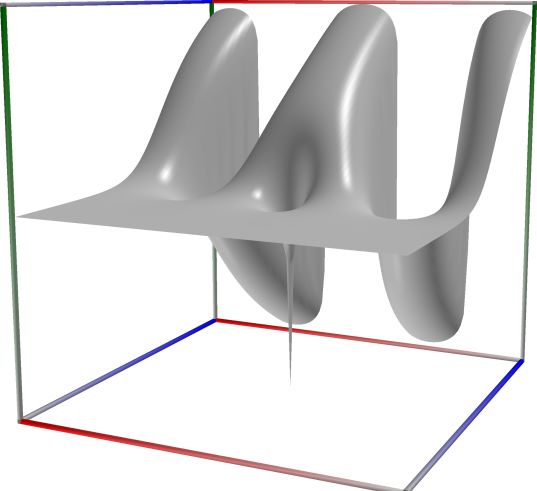
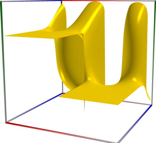
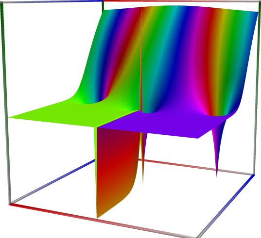
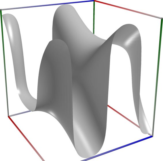
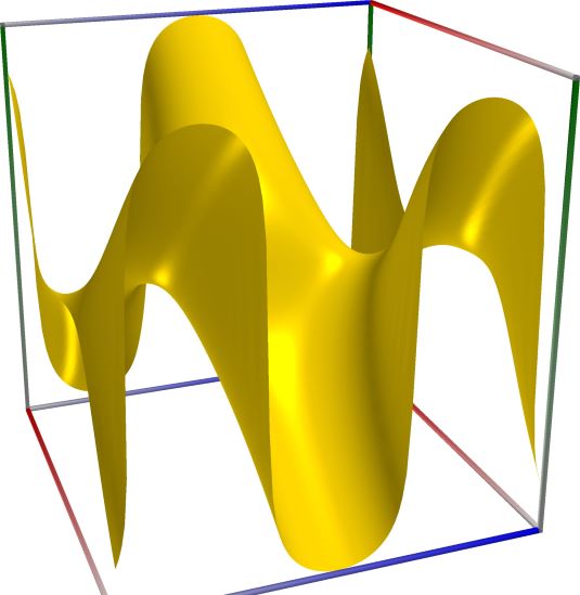
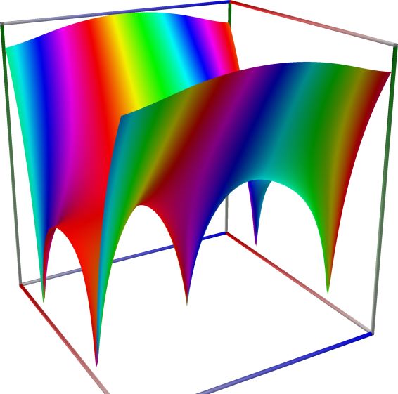
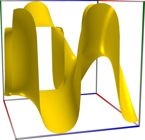
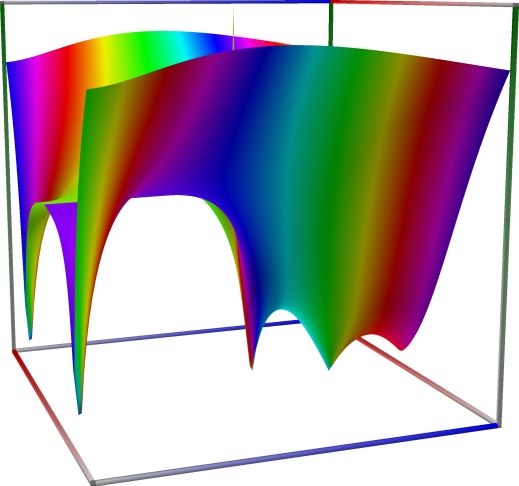
06a_TestEi_re \(\quad\) 06b_TestEi_im \(\quad\) 06c_TestEi_abs

Left figure: real part of the Ei function. Camera angles are \(\theta=135^\circ\) and \(\phi = -12^\circ\), camera radius is -2.

Middle figure: imaginary part of the Ei function. Camera angles are \(\theta=135^\circ\) and \(\phi = -12^\circ\), camera radius is -2.

Right figure: absolute value of the Ei function, with color-coded phase. Camera angles are \(\theta=135^\circ\) and \(\phi = -12^\circ\), camera radius is -2.

An example in Python

>>> from xlcalcnet import xreal
>>> xreal.Ei(0.5)
xreal('5.2359877559829887307E-1')
>>> xreal.Ei('0.51')
xreal('5.3518479027559984754E-1')

An example in Visual Basic

>>> from xlcalcnet import Gpr
>>> Gpr.Ei(0.5)
Gpr('5.2359877559829887307E-1')
>>> Gpr.Ei('0.51')
Gpr('5.3518479027559984754E-1')

An example with real input:

>>> from xlcalcnet import dec, mpm, gmp, fpm, apm
>>> mpm.dps = 40; x = 3.0
>>> \mathrm{d}x = dec.ei(x); mx = mpm.ei(x); gx = gmp.ei(x)
>>> fx = fpm.ei(x); ax = apm.ei(x)
>>> mpm.show([\mathrm{d}x, mx, gx, fx, ax])
dec:  9.933832570625416558008336019216765262991E+0
mpm:  9.933832570625416558008336019216765262991e+0
gmp:  9.933832570625416558008336019216765262991E+00
fpm:  9.93383257062542E+00
apm:  9.933832570625416558008336019216765262991e+0 (9.245e-40%)

An example with complex input:

>>> from xlcalcnet import dec, mpm, gmp, fpm, apm
>>> mpm.dps = 20; z = '3.0 + 4.0j'
>>> \mathrm{d}z = dec.ei(z); mz = mpm.ei(z); gz = gmp.ei(z)
>>> fz = fpm.ei(z); az = apm.ei(z)
>>> mpm.show([\mathrm{d}z, mz, gz, fz, az], aligned=True)
dec: -4.1540916516426898225E+0               + 4.2944186200243574770E+0j
mpm: -4.1540916516426898225e+0               + 4.2944186200243574770e+0j
gmp: -4.1540916516426898225E+00              + 4.2944186200243574770E+00j
fpm: -4.15409165164269E+00                   + 4.29441862002436E+00j
apm: -4.1540916516426898225e+0 (-8.156e-20%) + 4.2944186200243574770e+0 (7.89e-20%)j

Logarithmic integral \(\mathrm{li}(x)\)#

ctx.log_integral(z)#

where ctx is math53, mathc53 or ctxflint.

Also: math53.li(z), mathc53.Li(z), ctx.logIntegral(z)

Returns the logarithmic integral \(\displaystyle \mathrm{li}(x) = PV \int_{0}^{x} \frac{1}{\log(t)} \, \mathrm{d}t, \quad (x \neq 1)\). For \(x \neq 0\) the integral is calculated as \(\mathrm{li}(x)=\mathrm{Ei}(\log(x))\).

See also Wikipedia [1436], MathWorld [1063], NIST [847], Ehrhardt [309] (3.4.15), Ehrhardt [309] (4.2.40), Flint [839], Flint [832], Mpmath [691].

This function returns the logarithmic integral \(\text{li}(x)\) for \(x \geq 0\)

\[\text{li}(x) = PV \int_{0}^{x} \frac{1}{\log(t)} \mathrm{d}t, \quad (x \neq 1).\]

For \(x \neq 0\) the integral is calculated as \(\text{li}(x)=\text{Ei}(\log(x))\).
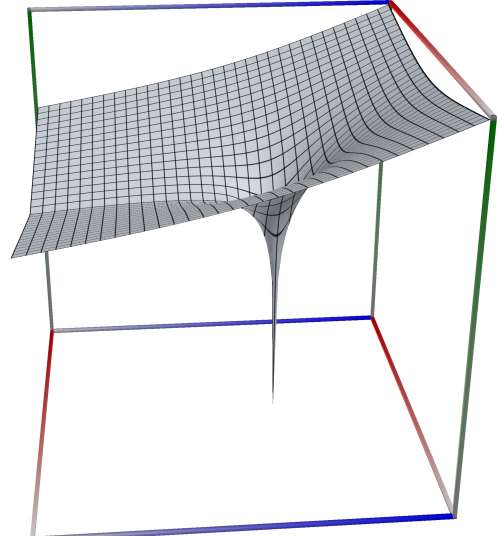
07a_TestLi_re \(\quad\) 07b_TestLi_im \(\quad\) 07c_TestLi_abs

Left figure: real part of the Li function. Camera angles are \(\theta=135^\circ\) and \(\phi = -12^\circ\), camera radius is -2.

Middle figure: imaginary part of the Li function. Camera angles are \(\theta=135^\circ\) and \(\phi = -12^\circ\), camera radius is -2.

Right figure: absolute value of the Li function, with color-coded phase. Camera angles are \(\theta=135^\circ\) and \(\phi = -12^\circ\), camera radius is -2.

An example in Python

>>> from xlcalcnet import xreal
>>> xreal.Li(0.5)
xreal('5.2359877559829887307E-1')
>>> xreal.Li('0.51')
xreal('5.3518479027559984754E-1')

An example in Visual Basic

>>> from xlcalcnet import Gpr
>>> Gpr.Li(0.5)
Gpr('5.2359877559829887307E-1')
>>> Gpr.Li('0.51')
Gpr('5.3518479027559984754E-1')

An example with real input:

>>> from xlcalcnet import dec, mpm, gmp, fpm, apm
>>> mpm.dps = 40; x = 3.0
>>> \mathrm{d}x = dec.li(x); mx = mpm.li(x); gx = gmp.li(x)
>>> fx = fpm.li(x); ax = apm.li(x)
>>> mpm.show([\mathrm{d}x, mx, gx, fx, ax])
dec:  2.163588594667191972876922367347721366542E+0
mpm:  2.163588594667191972876922367347721366542e+0
gmp:  2.163588594667191972876922367347721366542E+00
fpm:  2.16358859466719E+00
apm:  2.163588594667191972876922367347721366542e+0 (1.061e-39%)

An example with complex input:

>>> from xlcalcnet import dec, mpm, gmp, fpm, apm
>>> mpm.dps = 20; z = '3.0 + 4.0j'
>>> \mathrm{d}z = dec.li(z); mz = mpm.li(z); gz = gmp.li(z)
>>> fz = fpm.li(z); az = apm.li(z)
>>> mpm.show([\mathrm{d}z, mz, gz, fz, az], aligned=True)
dec: 3.1343755504645775265E+0              + 2.6769247817778742392E+0j
mpm: 3.1343755504645775265e+0              + 2.6769247817778742392e+0j
gmp: 3.1343755504645775265E+00             + 2.6769247817778742392E+00j
fpm: 3.13437555046458E+00                  + 2.67692478177787E+00j
apm: 3.1343755504645775265e+0 (1.081e-19%) + 2.6769247817778742392e+0 (6.328e-20%)j

Hyperbolic sine integral \(\mathrm{Shi}(x)\)#

ctx.sinh_integral(z)#

where ctx is math53, ctxflint.

Also: math53.shi(z), ctx.sinhIntegral(z)

Returns the hyperbolic sine integral \(\displaystyle \mathrm{Shi}(x) = \int_0^x \frac{\sinh(t)}{t} \, \mathrm{d}t\), and \(\mathrm{Shi}(x) = -\mathrm{Shi}(-x)\) for \(x<0\).

See also Wikipedia [1433], MathWorld [1059], NIST [846], Ehrhardt [309] (3.4.17), Flint [839], Flint [832], Mpmath [694].

This function returns the hyperbolic sine integral

\[\text{Shi}(x) = \int_0^x \frac{\sinh(t)}{t} \mathrm{d}t,\]

and \(\text{Shi}(x) = -\text{Shi}(-x)\) for \(x<0\). The integral is calculated using the relation

\[\text{Shi}(x) = \tfrac{1}{2} \left(\text{Ei}(x)+\text{E}_1(x)\right), \quad (x>0).\]
\[\text{Shi}(x) = -i \text{Si}(ix).\]

An example in Python

>>> from xlcalcnet import xreal
>>> xreal.Shi(0.5)
xreal('5.2359877559829887307E-1')
>>> xreal.Shi('0.51')
xreal('5.3518479027559984754E-1')

An example in Visual Basic

>>> from xlcalcnet import Gpr
>>> Gpr.Shi(0.5)
Gpr('5.2359877559829887307E-1')
>>> Gpr.Shi('0.51')
Gpr('5.3518479027559984754E-1')

An example with real input:

>>> from xlcalcnet import dec, mpm, gmp, fpm, apm
>>> mpm.dps = 40; x = 3.0
>>> \mathrm{d}x = dec.shi(x); mx = mpm.shi(x); gx = gmp.shi(x)
>>> fx = fpm.shi(x); ax = apm.shi(x)
>>> mpm.show([\mathrm{d}x, mx, gx, fx, ax])
dec:  4.973440475859806797710418382522705142970E+0
mpm:  4.973440475859806797710418382522705142970e+0
gmp:  4.973440475859806797710418382522705142970E+00
fpm:  4.97344047585981E+00
apm:  4.973440475859806797710418382522705142970e+0 (9.233e-40%)

An example with complex input:

>>> from xlcalcnet import dec, mpm, gmp, fpm, apm
>>> mpm.dps = 20; z = '3.0 + 4.0j'
>>> \mathrm{d}z = dec.shi(z); mz = mpm.shi(z); gz = gmp.shi(z)
>>> fz = fpm.shi(z); az = apm.shi(z)
>>> mpm.show([\mathrm{d}z, mz, gz, fz, az], aligned=True)
dec: -2.0766138488418551187E+0               + 2.1516024142007774595E+0j
mpm: -2.0766138488418551187e+0               + 2.1516024142007774595e+0j
gmp: -2.0766138488418551187E+00              + 2.1516024142007774595E+00j
fpm: -2.07661384884186E+00                   + 2.15160241420078E+00j
apm: -2.0766138488418551187e+0 (-1.632e-19%) + 2.1516024142007774595e+0 (7.874e-20%)j

Hyperbolic cosine integral \(\mathrm{Chi}(x)\)#

ctx.cosh_integral(z)#

where ctx is math53, ctxflint.

Note: Also math53.chi(z), ctx.coshIntegral(z)

Returns the hyperbolic cosine integral \(\displaystyle \mathrm{Chi}(x) = -\int_x^{\infty} \frac{\cosh(t)}{t} \, \mathrm{d}t = \gamma + \log(x) + \int_0^x \frac{\cosh(t) - 1}{t} \, \mathrm{d}t\).

See also Wikipedia [1432], MathWorld [1058], NIST [846], Ehrhardt [309] (3.4.1), Flint [839], Flint [832], Mpmath [678].

The hyperbolic cosine integral is defined as

\[\text{Chi}(x) = \gamma + \log(x) + \int_0^x \frac{\cosh(t)-1}{t} \mathrm{d}t,\]

and \(\text{Chi}(x) = \text{Chi}(-x)\) for \(x<0\). The integral is calculated using the relation

\[\text{Chi}(x) = \tfrac{1}{2} \left(\text{Ei}(x)-\text{E}_1(x)\right), \quad (x>0).\]

We also have

\[\text{Chi}(x) = \text{Ci}(i x) - \log(i x) + \log(x).\]

and

\[\mathrm{Chi}(z) = -\frac{1}{2} \left[ e^{z} U(1,1,-z) + e^{-z} U(1,1,z) + \log(-z) - \log(z) \right]\]

An example in Python

>>> from xlcalcnet import xreal
>>> xreal.Chi(0.5)
xreal('5.2359877559829887307E-1')
>>> xreal.Chi('0.51')
xreal('5.3518479027559984754E-1')

An example in Visual Basic

>>> from xlcalcnet import Gpr
>>> Gpr.Chi(0.5)
Gpr('5.2359877559829887307E-1')
>>> Gpr.Chi('0.51')
Gpr('5.3518479027559984754E-1')

An example with real input:

>>> from xlcalcnet import dec, mpm, gmp, fpm, apm
>>> mpm.dps = 40; x = 3.0
>>> \mathrm{d}x = dec.chi(x); mx = mpm.chi(x); gx = gmp.chi(x)
>>> fx = fpm.chi(x); ax = apm.chi(x)
>>> mpm.show([\mathrm{d}x, mx, gx, fx, ax])
dec:  4.960392094765609760297917636694060120021E+0
mpm:  4.960392094765609760297917636694060120021e+0
gmp:  4.960392094765609760297917636694060120021E+00
fpm:  4.96039209476561E+00
apm:  4.960392094765609760297917636694060120020e+0 (6.387e-38%)

An example with complex input:

>>> from xlcalcnet import dec, mpm, gmp, fpm, apm
>>> mpm.dps = 20; z = '3.0 + 4.0j'
>>> \mathrm{d}z = dec.chi(z); mz = mpm.chi(z); gz = gmp.chi(z)
>>> fz = fpm.chi(z); az = apm.chi(z)
>>> mpm.show([\mathrm{d}z, mz, gz, fz, az], aligned=True)
dec: -2.0774778028008347038E+0               + 2.1428162058235800175E+0j
mpm: -2.0774778028008347038e+0               + 2.1428162058235800175e+0j
gmp: -2.0774778028008347038E+00              + 2.1428162058235800175E+00j
fpm: -2.07747780280083E+00                   + 2.14281620582358E+00j
apm: -2.0774778028008347038e+0 (-1.631e-19%) + 2.1428162058235800175e+0 (1.581e-19%)j

Generalized exponential integral \(E_n(x)\)#

ctx.exp_integral_en(n, z)#

where ctx is math53, ctxboost or ctxflint.

Note: math53.en(n, x)

Returns the generalized exponential integral of integer order \(\displaystyle E_n(x) = \int_{1}^{\infty} \frac{e^{-xt}}{t^n} \, \mathrm{d}t\).

See also Wikipedia [1427], MathWorld [1053], NIST [485], BoostMath [161], Ehrhardt [309] (3.4.12), Mpmath [684].

The exponential integrals \(\text{E}_n(x)\) of integer order is defined as

\[\text{E}_n(x) = \int_{1}^{\infty} \frac{e^{-xt}}{t^n} \mathrm{d}t, \quad (n \geq 0).\]

For \(x<0\) the integral is calculated as \(\text{Ei}(x) = -\text{E}_1(-x)\).

!!Note: check syntax in mpmath!!

Returns gives the generalized exponential integral or En-function,

\[\mathrm{E}_n(z) = \int_1^{\infty} \frac{e^{-zt}}{t^n} \mathrm{d}t,\]
\[\text{E}_n(1-s) = z^{-s} \Gamma(s,z).\]

An example in Python

>>> from xlcalcnet import xreal
>>> xreal.En(3, 0.5)
xreal('5.2359877559829887307E-1')
>>> xreal.En(3, '0.51')
xreal('5.3518479027559984754E-1')

An example in Visual Basic

>>> from xlcalcnet import Gpr
>>> Gpr.En(3, 0.5)
Gpr('5.2359877559829887307E-1')
>>> Gpr.En(3, '0.51')
Gpr('5.3518479027559984754E-1')

An example with real input:

>>> from xlcalcnet import dec, mpm, gmp, fpm, apm
>>> mpm.dps = 40; n = '4'; x = '5.0'
>>> \mathrm{d}x = dec.expint(n, x); mx = mpm.expint(n, x); gx = gmp.expint(n, x)
>>> fx = fpm.expint(n, x); ax = apm.expint(n, x)
>>> mpm.show([\mathrm{d}x, mx, gx, fx, ax])
dec:  7.829808450774252432788031803000123235715E-4
mpm:  7.829808450774252432788031803000123235715e-4
gmp:  7.829808450774252432788031803000123235715E-04
fpm:  7.82980845077425E-04
apm:  7.829808450774252432788031803000123235723e-4 (2.172e-36%)

An example with complex input:

>>> from xlcalcnet import dec, mpm, gmp, fpm, apm
>>> mpm.dps = 20; n = '4'; z = '5.0 + 3.0j'
>>> \mathrm{d}z = dec.expint(n, z); mz = mpm.expint(n, z); gz = gmp.expint(n, z)
>>> fz = fpm.expint(n, z); az = apm.expint(n, z)
>>> mpm.show([\mathrm{d}z, mz, gz, fz, az], aligned=True)
dec: -7.1820162264651649511E-4               + 1.4860820449934938829E-4j
mpm: -7.1820162264651649511e-4               + 1.4860820449934938829e-4j
gmp: -7.1820162264651649511E-04              + 1.4860820449934938829E-04j
fpm: -7.18201622646517E-04                   + 1.48608204499349E-04j
apm: -7.1820162264651649571e-4 (-1.103e-15%) + 1.4860820449934939066e-4 (8.075e-15%)j

Sine integral \(\mathrm{Si}(x)\)#

ctx.sin_integral(z)#

where ctx is math53, ctxflint.

Also: math53.si(z), ctx.sinIntegral(z)

Returns the sine integral \(\displaystyle \mathrm{Si}(x) = \int_0^x \frac{\sin(t)}{t} \, \mathrm{d}t\), and \(\mathrm{Si}(x) = -\mathrm{Si}(-x)\) for \(x<0\).

See also Wikipedia [1441], MathWorld [1065], NIST [849], Ehrhardt [309] (3.4.18), Flint [839], Flint [832], Mpmath [695].

This function returns the sine integral

\[\text{Si}(x) = \int_0^x \frac{\sin(t)}{t} \mathrm{d}t,\]

and \(\text{Si}(x) = -\text{Si}(-x)\) for \(x<0\).

Computes the sine integral \(\mathrm{Si}(z)\), respectively using

\[\mathrm{Si}(z) = \frac{i}{2} \left[ e^{iz} U(1,1,-iz) - e^{-iz} U(1,1,iz) + \log(-iz) - \log(iz) \right]\]
\[\mathrm{Si}(z) = z {}_1F_2(\tfrac{1}{2}; \tfrac{3}{2}, \tfrac{3}{2}; -\tfrac{z^2}{4})\]

and an automatic algorithm choice.

13a_TestSinIntegral_re \(\quad\) 13b_TestSinIntegral_im \(\quad\) 13c_TestSinIntegral_abs

Left figure: real part of the Sine integral \(\mathrm{Si}(x)\). Camera angles are \(\theta=135^\circ\) and \(\phi = -12^\circ\), camera radius is -2.

Middle figure: imaginary part of the Sine integral \(\mathrm{Si}(x)\). Camera angles are \(\theta=135^\circ\) and \(\phi = -12^\circ\), camera radius is -2.

Right figure: absolute value of the Sine integral \(\mathrm{Si}(x)\), with color-coded phase. Camera angles are \(\theta=135^\circ\) and \(\phi = -12^\circ\), camera radius is -2.

An example in Python

>>> from xlcalcnet import xreal
>>> xreal.Si(0.5)
xreal('5.2359877559829887307E-1')
>>> xreal.Si('0.51')
xreal('5.3518479027559984754E-1')

An example in Visual Basic

>>> from xlcalcnet import Gpr
>>> Gpr.Si(0.5)
Gpr('5.2359877559829887307E-1')
>>> Gpr.Si('0.51')
Gpr('5.3518479027559984754E-1')

An example with real input:

>>> from xlcalcnet import dec, mpm, gmp, fpm, apm
>>> mpm.dps = 40; x = 3.0
>>> \mathrm{d}x = dec.si(x); mx = mpm.si(x); gx = gmp.si(x)
>>> fx = fpm.si(x); ax = apm.si(x)
>>> mpm.show([\mathrm{d}x, mx, gx, fx, ax])
dec:  1.848652527999468256397730251111973245165E+0
mpm:  1.848652527999468256397730251111973245165e+0
gmp:  1.848652527999468256397730251111973245165E+00
fpm:  1.84865252799947E+00
apm:  1.848652527999468256397730251111973245165e+0 (6.21e-40%)

An example with complex input:

>>> from xlcalcnet import dec, mpm, gmp, fpm, apm
>>> mpm.dps = 20; z = '3.0 + 4.0j'
>>> \mathrm{d}z = dec.si(z); mz = mpm.si(z); gz = gmp.si(z)
>>> fz = fpm.si(z); az = apm.si(z)
>>> mpm.show([\mathrm{d}z, mz, gz, fz, az], aligned=True)
dec: 6.7479950814040320927E+0              - 3.4986637211319094706E+0j
mpm: 6.7479950814040320927e+0              - 3.4986637211319094706e+0j
gmp: 6.7479950814040320927E+00             - 3.4986637211319094706E+00j
fpm: 6.74799508140403E+00                  - 3.49866372113191E+00j
apm: 6.7479950814040320927e+0 (1.004e-19%) - 3.4986637211319094706e+0 (-4.842e-20%)j

Cosine integral \(\mathrm{Ci}(x)\)#

ctx.cos_integral(z)#

where ctx is math53 or ctxflint.

Note: Also math53.ci(z), ctx.cosIntegral(z)

Returns the cosine integral \(\displaystyle \mathrm{Ci}(x) = -\int_x^{\infty} \frac{\cos(t)}{t} \, \mathrm{d}t = \gamma + \log(x) + \int_0^x \frac{\cos(t) - 1}{t} \, \mathrm{d}t\).

See also Wikipedia [1426], MathWorld [1046], NIST [849], Ehrhardt [309] (3.4.2), Flint [839], Flint [832], Mpmath [681].
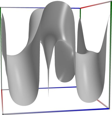
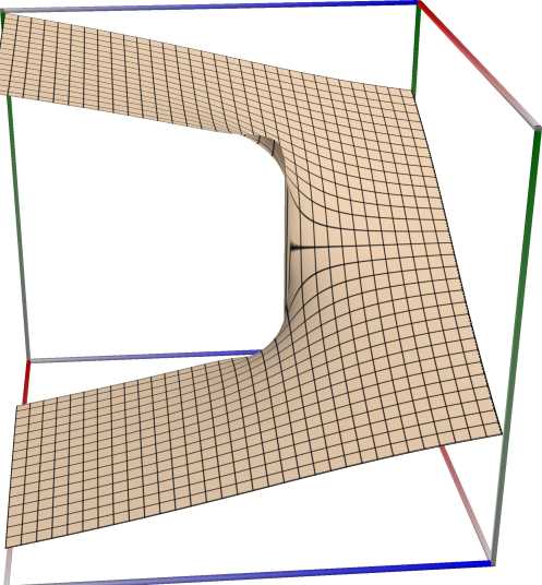
12a_TestCosIntegral_re \(\quad\) 12b_TestCosIntegral_im \(\quad\) 12c_TestCosIntegral_abs

Left figure: real part of the Cosine integral \(\mathrm{Ci}(x)\). Camera angles are \(\theta=135^\circ\) and \(\phi = -12^\circ\), camera radius is -2.

Middle figure: imaginary part of the Cosine integral \(\mathrm{Ci}(x)\). Camera angles are \(\theta=135^\circ\) and \(\phi = -12^\circ\), camera radius is -2.

Right figure: absolute value of the Cosine integral \(\mathrm{Ci}(x)\), with color-coded phase. Camera angles are \(\theta=135^\circ\) and \(\phi = -12^\circ\), camera radius is -2.

The cosine integral is defined as

\[\text{Ci}(x) = \gamma + \log(x) + \int_0^x \frac{\cos(t)-1}{t} \mathrm{d}t,\]

and \(\text{Ci}(x) = \text{Ci}(-x)\) for \(x<0\).

Computes the cosine integral \(\mathrm{Ci}(z)\), respectively using

\[\mathrm{Ci}(z) = \log(z) - \frac{1}{2} \left[ e^{iz} U(1,1,-iz) + e^{-iz} U(1,1,iz) + \log(-iz) + \log(iz) \right]\]
\[\mathrm{Ci}(z) = -\tfrac{z^2}{4} {}_2F_3(1, 1; 2, 2, \tfrac{3}{2}; -\tfrac{z^2}{4}) + \log(z) + \gamma\]

and an automatic algorithm choice.

An example in Python

>>> from xlcalcnet import xreal
>>> xreal.Ci(0.5)
xreal('5.2359877559829887307E-1')
>>> xreal.Ci('0.51')
xreal('5.3518479027559984754E-1')

An example in Visual Basic

>>> from xlcalcnet import Gpr
>>> Gpr.Ci(0.5)
Gpr('5.2359877559829887307E-1')
>>> Gpr.Ci('0.51')
Gpr('5.3518479027559984754E-1')

An example with real input:

>>> from xlcalcnet import dec, mpm, gmp, fpm, apm
>>> mpm.dps = 40; x = 3.0
>>> \mathrm{d}x = dec.ci(x); mx = mpm.ci(x); gx = gmp.ci(x)
>>> fx = fpm.ci(x); ax = apm.ci(x)
>>> mpm.show([\mathrm{d}x, mx, gx, fx, ax])
dec:  1.196297860080003276264722811766778505468E-1
mpm:  1.196297860080003276264722811766778505468e-1
gmp:  1.196297860080003276264722811766778505468E-01
fpm:  1.19629786008000E-01
apm:  1.196297860080003276264722811766778505468e-1 (1.799e-39%)

An example with complex input:

>>> from xlcalcnet import dec, mpm, gmp, fpm, apm
>>> mpm.dps = 20; z = '3.0 + 4.0j'
>>> \mathrm{d}z = dec.ci(z); mz = mpm.ci(z); gz = gmp.ci(z)
>>> fz = fpm.ci(z); az = apm.ci(z)
>>> mpm.show([\mathrm{d}z, mz, gz, fz, az], aligned=True)
dec: -3.4957570339825683441E+0               - 5.1759052151768084089E+0j
mpm: -3.4957570339825683441e+0               - 5.1759052151768084089e+0j
gmp: -3.4957570339825683441E+00              - 5.1759052151768084089E+00j
fpm: -3.49575703398257E+00                   - 5.17590521517681E+00j
apm: -3.4957570339825683441e+0 (-9.692e-20%) - 5.1759052151768084089e+0 (-6.546e-20%)j

previous

Error function and related functions

next

Hypergeometric functions \(\,_2F_1\) and \(\,_1F_2\) (and related functions)

Contents
  • Exponential integral \(E_1(x)\)
    • ctx.exp_integral_e1()
  • Exponential integral \(\mathrm{Ei}(x)\)
    • ctx.exp_integral_ei()
  • Logarithmic integral \(\mathrm{li}(x)\)
    • ctx.log_integral()
  • Hyperbolic sine integral \(\mathrm{Shi}(x)\)
    • ctx.sinh_integral()
  • Hyperbolic cosine integral \(\mathrm{Chi}(x)\)
    • ctx.cosh_integral()
  • Generalized exponential integral \(E_n(x)\)
    • ctx.exp_integral_en()
  • Sine integral \(\mathrm{Si}(x)\)
    • ctx.sin_integral()
  • Cosine integral \(\mathrm{Ci}(x)\)
    • ctx.cos_integral()

By Dietrich Hadler

© Copyright 2026, Dietrich Hadler. .

Last updated on Aug 19, 2026.