Weierstrass elliptic functions, in terms of (real) lattice invariants \(g_2, g_3\)#
The Weierstrass functions take real values on the real axis iff the lattice is fixed under complex conjugation, or, equivalently, when \(g_2, g_3 \in \mathbb{R}\).
See also: https://gist.github.com/stla/d771e0a8c351d16d186c79bc838b6c48
Weierstrass function \(\wp_g(z, g_2, g_3)\) (also DAMath)#
- ctxflint.weierstrass_p_g(z, g2, g3)#
Computes Weierstrass’s elliptic function \(\wp_g(z; g_2, g_3)\).
We have \(\wp_g(tz; t^{-4} g_2, t^{-6} g_3) = t^{-2} \wp_g(z; g_2, g_3)\) and \(\wp_g(i z; g_2, g_3) = -\wp_g(z; g_2, -g_3)\).
See also MathWorld [1066], Flint [837].
Returns the Weierstrass function \(\wp_g(x, g_2, g_3)\) based on the lattice invariants \(g_2\), \(g_3\).
In AMath the computation of the Weierstass elliptic function (for real and imaginary arguments) is based on the lattice invariants \(g_2\), \(g_3\) or the lattice roots \(e_1, e_2, e_3 = -e_1-e_2\), if the discriminant of the cubic equation \(4x^3 - g_2x - g_3 = 0\) is positive
\[\Delta = g_2^3 - 27g_3^2 = 16(e_2-e_3)^2 (e_3-e_1)^2 (e_1-e_2)^2;\]symbolically written as \(\wp_g(x, g_2, g_3)\) or \(\wp_e(x,e_1,e_2)\). See also
When \(g_2=1, g_3=0\) the result is \(\wp_l(x)\) and for \(g_2=g_3=0\) it is \(x-2\). If \(g_2^2 - 27g_3^2>0\) all lattice roots are real, and \(\wp'_e(x,e_1,e_2)\) is returned, otherwise the following Jacobi relation is used:
\[\wp_g(x, g_2, g_3) = e_2 + H \frac{1+\mathrm{cn}(u,k)}{1-\mathrm{cn}(u,k)} , \quad k = \sqrt{\tfrac{1}{2}\frac{3e_2}{4H}}, \quad u = 2x \sqrt{H}, \quad H = \sqrt{(e_2-e_1)(e_2-e_3)}.\]See also Wikipedia [1463], MathWorld [1066], Ehrhardt [309] (3.2.17.5).
Returns the Weierstrass function \(\wp_g(iy,g_2, g_3) = -\wp_g(y,g_2, -g_3)\). See also: MathWorld [1067], Ehrhardt [309] (3.2.17.7).
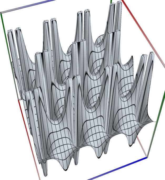 \(\quad\)
 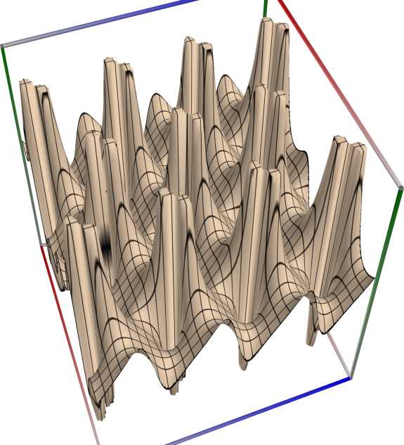 \(\quad\)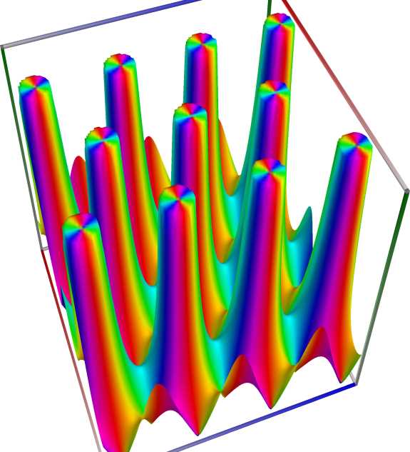
Left figure: real part of the Weierstrass function \(\wp_g(z, g_2, g_3)\). Camera angles are \(\theta=135^\circ\) and \(\phi = -12^\circ\), camera radius is -2.
Middle figure: imaginary part of the Weierstrass function \(\wp_g(z, g_2, g_3)\). Camera angles are \(\theta=135^\circ\) and \(\phi = -12^\circ\), camera radius is -2.
Right figure: absolute value of the Weierstrass function \(\wp_g(z, g_2, g_3)\), with color-coded phase. Camera angles are \(\theta=135^\circ\) and \(\phi = -12^\circ\), camera radius is -2.
For \(\Delta = g_2^3 - 27 g_3^2 \ne 0\), we first compute the elliptic half periods \(\omega_1, \omega_2\) from the lattice invariants \(g_2, g_3\) (see EllipticHalfPeriodsG), and set \(\omega = \omega_1, \tau = \omega_2/\omega_1\). Then \(\wp_g(z; g_2, g_3) = \wp(z| \omega, \tau)\) (see WeierstrassP).
For \(\Delta = 0, g_2 > 0, g_3 \ne 0\), the function \(\wp_g(\cdot)\) degenerates to a simply periodic function, which can be expressed in closed form in terms of elementary functions:
For \(\displaystyle \Delta = 0, g_2 > 0, g_3 < 0: \quad \wp_g(z; g_2, g_3) = c + \frac{3c}{\sinh^2\left(\sqrt{3c} z \right)}, \quad \text{where } c = \sqrt{g_2/12}\).
For \(\displaystyle \Delta = 0, g_2 > 0, g_3 > 0: \quad \wp_g(z; g_2, g_3) = c + \frac{3c}{\sin^2\left( \sqrt{3c}z \right)}, \quad \text{where } c = \sqrt{g_2/12}\).
If both \(g_2\) and \(g_3\) are zero, the function \(\wp_g(\cdot)\) degenerates to a function that is not periodic at all, namely \(\wp_g(z; 0, 0) = z^{-2}\).
An example with real input for \(z\) and with purely imaginary input for \(\tau\), producing real output:
>>> from xlcalcnet import dec, mpm, gmp, fpm, apm
>>> mpm.dps = 40; z = '0.1'; tau = '0.0 + 0.9j'
>>> \mathrm{d}x = dec.weierstrass_p(z, tau); mx = mpm.weierstrass_p(z, tau)
>>> gx = gmp.weierstrass_p(z, tau)
>>> fx = fpm.weierstrass_p(z, tau); ax = apm.weierstrass_p(z, tau)
>>> mpm.show([\mathrm{d}x, mx, gx, fx, ax])
dec:  1.001202913728593351620333736461324760825E+2
mpm:  1.001202913728593351620333736461324760825e+2
gmp:  1.001202913728593351620333736461324760825E+02
fpm:  1.00120291372859E+02
apm:  1.001202913728593351620333736461324760825e+2 (1.321e-38%)
An example with complex input for \(z\) and \(\tau\):
>>> from xlcalcnet import dec, mpm, gmp, fpm, apm
>>> mpm.dps = 20; z = '0.1 + 0.5j'; tau = '0.7 + 0.9j'
>>> \mathrm{d}x = dec.weierstrass_p(z, tau); mx = mpm.weierstrass_p(z, tau)
>>> gx = gmp.weierstrass_p(z, tau)
>>> fx = fpm.weierstrass_p(z, tau); ax = apm.weierstrass_p(z, tau)
>>> mpm.show([\mathrm{d}x, mx, gx, fx, ax], aligned=True)
dec:  -2.3859027427781674104E+0
mpm:  -2.3859027427781674104e+0
gmp:  -2.3859027427781674104E+00
fpm:  -2.38590274277817E+00
apm:  (-2.3859027427781674104e+0 (-2.038e-17%) + 2.4323666240267878020e-2 (1.982e-15%)j)
Weierstrass function, first derivative: \(\wp_g'(z, g_2, g_3)\)#
- ctxflint.weierstrass_p_prime_(z, g2, g3)#
Computes the first derivative of the Weierstrass function, \(\wp_g'(z, g_2, g_3)\).
We have \(\wp_g'(tz; t^{-4} g_2, t^{-6} g_3) = t^{-3} \wp_g'(z; g_2, g_3)\) and \(\wp_g'(i z; g_2, g_3) = i\wp_g'(z; g_2, -g_3)\).
See also MathWorld [1067], Flint [837].
Returns the Weierstrass function \(\wp_g(x, g_2, g_3)\) based on the lattice invariants \(g_2\), \(g_3\).
\[\wp'_g(x, g_2, g_3) = -H^{3/2} \frac{\mathrm{cn}(u,k)\mathrm{dn}(u,k)}{1-\mathrm{cn}(u,k)} , \quad k = \sqrt{\tfrac{1}{2}\frac{3e_2}{4H}}, \quad u = 2x \sqrt{H}, \quad H = \sqrt{(e_2-e_1)(e_2-e_3)}.\]
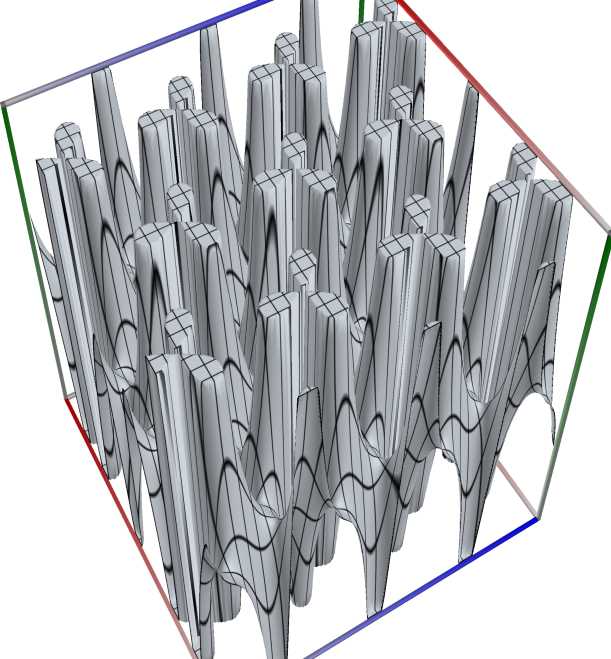 \(\quad\)
  \(\quad\)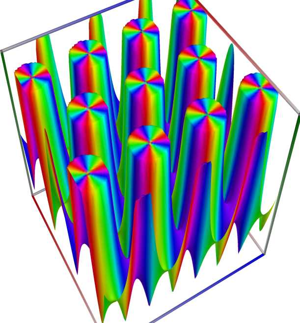
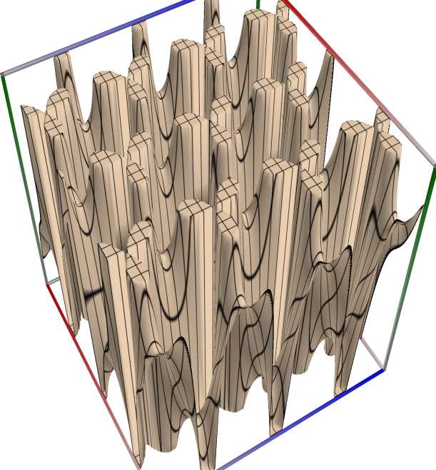
Left figure: real part of the Weierstrass function, first derivative: \(\wp_g'(z, g_2, g_3)\). Camera angles are \(\theta=135^\circ\) and \(\phi = -12^\circ\), camera radius is -2.
Middle figure: imaginary part of the Weierstrass function, first derivative: \(\wp_g'(z, g_2, g_3)\). Camera angles are \(\theta=135^\circ\) and \(\phi = -12^\circ\), camera radius is -2.
Right figure: absolute value of the Weierstrass function, first derivative: \(\wp_g'(z, g_2, g_3)\), with color-coded phase. Camera angles are \(\theta=135^\circ\) and \(\phi = -12^\circ\), camera radius is -2.
For \(\Delta = g_2^3 - 27 g_3^2 \ne 0\), we first compute the elliptic half periods \(\omega_1, \omega_2\) from the lattice invariants \(g_2, g_3\) (see EllipticHalfPeriodsG), and set \(\omega = \omega_1, \tau = \omega_2/\omega_1\). Then \(\wp_g'(z; g_2, g_3) = \wp'(z| \omega, \tau)\) (see WeierstrassPPrime).
For \(\Delta = 0, g_2 > 0, g_3 \ne 0\), the function \(\wp_g'(\cdot)\) degenerates to a simply periodic function, which can be expressed in closed form in terms of elementary functions:
For \(\Delta = 0, g_2 > 0, g_3 < 0: \quad \displaystyle \wp_g'(z; g_2, g_3) = -6 \sqrt{3} c^{3/2} \mathrm{coth}(\sqrt{3c}z) \mathrm{csch}^2(\sqrt{3c}z), \quad \text{where } c = \sqrt{g_2/12}\).
For \(\Delta = 0, g_2 > 0, g_3 > 0: \quad \displaystyle \wp_g'(z; g_2, g_3) = -6 \sqrt{3} c^{3/2} \mathrm{cot}(\sqrt{3c}z) \mathrm{csc}^2(\sqrt{3c}z), \quad \text{where } c = \sqrt{g_2/12}\).
If both \(g_2\) and \(g_3\) are zero, the function \(\wp_g'(\cdot)\) degenerates to a function that is not periodic at all, namely \(\wp_g'(z; 0, 0) = -2 z^{-3}\).
An example with real input for \(z\) and with purely imaginary input for \(\tau\), producing real output:
>>> from xlcalcnet import dec, mpm, gmp, fpm, apm
>>> mpm.dps = 40; z = '0.1'; tau = '0.0 + 0.9j'
>>> \mathrm{d}x = dec.weierstrass_p_prime(z, tau); mx = mpm.weierstrass_p_prime(z, tau)
>>> gx = gmp.weierstrass_p_prime(z, tau)
>>> fx = fpm.weierstrass_p_prime(z, tau); ax = apm.weierstrass_p_prime(z, tau)
>>> mpm.show([\mathrm{d}x, mx, gx, fx, ax])
dec:  -1.997612036772329460780279347633189585828E+3
mpm:  -1.997612036772329460780279347633189585828e+3
gmp:  -1.997612036772329460780279347633189585828E+03
fpm:  -1.99761203677233E+03
apm:  -1.997612036772329460780279347633189585828e+3 (-1.883e-38%)
An example with complex input for \(z\) and \(\tau\):
>>> from xlcalcnet import dec, mpm, gmp, fpm, apm
>>> mpm.dps = 20; z = '0.1 + 0.5j'; tau = '0.7 + 0.9j'
>>> \mathrm{d}x = dec.weierstrass_p_prime(z, tau); mx = mpm.weierstrass_p_prime(z, tau)
>>> gx = gmp.weierstrass_p_prime(z, tau)
>>> fx = fpm.weierstrass_p_prime(z, tau); ax = apm.weierstrass_p_prime(z, tau)
>>> mpm.show([\mathrm{d}x, mx, gx, fx, ax], aligned=True)
dec: 1.4787544521497118400E+1
mpm: 1.4787544521497118400e+1
gmp: 1.4787544521497118400E+01
fpm: 1.47875445214971E+01
apm: 1.4787544521497118399e+1 (5.664e-17%) - 2.3205214399360215619e+1 (-3.609e-17%)j
Inverse Weierstrass function \(\wp_g^{-1}(z, g_2, g_3)\)#
- ctxflint.weierstrass_p_invG(z, g2, g3)#
Computes the Inverse Weierstrass function \(\wp_g^{-1}(z, g_2, g_3)\)
See also MathWorld [1062], Flint [837].
\[\wp_g^{-1}(z; g_2, g_3) = \wp^{-1}(z| \tau = \omega_2/\omega_1, \omega = \omega_1)\]Returns the functional inverse \(\wp^{-1}_g\) of the Weierstrass function for \(y \ge e_1\), i.e. the smallest positive \(x\) with \(\wp^{-1}_g(y,g_2,g_3) = y\), if it exists. See also: MathWorld [1062], Ehrhardt [309] (3.2.17.9).
An example with real input for \(z\) and with purely imaginary input for \(\tau\), producing real output:
>>> from xlcalcnet import dec, mpm, gmp, fpm, apm
>>> mpm.dps = 40; z = '100'; tau = '0.0 + 0.9j'
>>> \mathrm{d}x = dec.weierstrass_p_inv(z, tau); mx = mpm.weierstrass_p_inv(z, tau)
>>> gx = gmp.weierstrass_p_inv(z, tau)
>>> fx = fpm.weierstrass_p_inv(z, tau); ax = apm.weierstrass_p_inv(z, tau)
>>> mpm.show([\mathrm{d}x, mx, gx, fx, ax])
dec:  1.000602721184701332310197413726890982085E-1
mpm:  1.000602721184701332310197413726890982085e-1
gmp:  1.000602721184701332310197413726890982085E-01
fpm:  1.00060272118470E-01
apm:  1.000602721184701332310197413726890982085e-1 (7.17e-40%)
An example with complex input for \(z\) and \(\tau\):
>>> from xlcalcnet import dec, mpm, gmp, fpm, apm
>>> mpm.dps = 20; z = '0.1 + 0.5j'; tau = '0.7 + 0.9j'
>>> \mathrm{d}x = dec.weierstrass_p_inv(z, tau); mx = mpm.weierstrass_p_inv(z, tau)
>>> gx = gmp.weierstrass_p_inv(z, tau)
>>> fx = fpm.weierstrass_p_inv(z, tau); ax = apm.weierstrass_p_inv(z, tau)
>>> mpm.show([\mathrm{d}x, mx, gx, fx, ax], aligned=True)
dec: 4.2630465458606458544E-1              - 3.0967048559182771279E-1j
mpm: 4.2630465458606458544e-1              - 3.0967048559182771279e-1j
gmp: 4.2630465458606458544E-01             - 3.0967048559182771279E-01j
fpm: 4.26304654586065E-01                  - 3.09670485591828E-01j
apm: 4.2630465458606458544e-1 (1.265e-16%) - 3.0967048559182771279e-1 (-1.063e-16%)j
Weierstrass Zeta function \(\zeta_g(z, g_2, g_3)\)#
- ctxflint.weierstrass_zeta_g(z, g2, g3)#
Computes the Weierstrass zeta function \(\zeta_g(z; g_2, g_3)\).
We have \(\zeta_g(tz; t^{-4} g_2, t^{-6} g_3) = t^{-1} \zeta_g(z; g_2, g_3)\) and \(\zeta_g(i z; g_2, g_3) = -i\zeta_g(z; g_2, -g_3)\).
The function is related to \(\wp(z; g_2, g_3)\) by \(\displaystyle \frac{d \zeta(z; g_2, g_3)}{\mathrm{d}z} = -\wp(z; g_2, g_3)\) and \(\displaystyle \zeta(z; g_2, g_3) - z^{-1} = \int_0^z \left(\wp(z; g_2, g_3) - z^{-2} \right)\).
 \(\quad\)
  \(\quad\)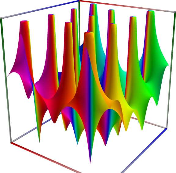
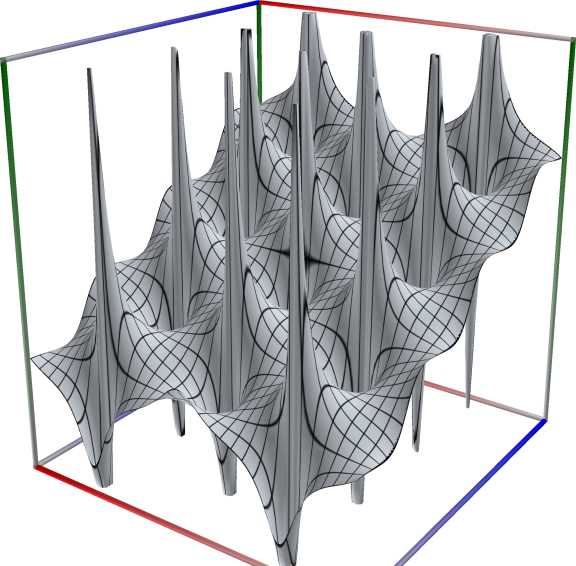
Left figure: real part of the Weierstrass Zeta function \(\zeta_g(z, g_2, g_3)\). Camera angles are \(\theta=135^\circ\) and \(\phi = -12^\circ\), camera radius is -2.
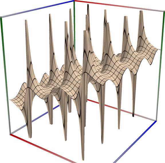
Middle figure: imaginary part of the Weierstrass Zeta function \(\zeta_g(z, g_2, g_3)\). Camera angles are \(\theta=135^\circ\) and \(\phi = -12^\circ\), camera radius is -2.
Right figure: absolute value of the Weierstrass Zeta function \(\zeta_g(z, g_2, g_3)\), with color-coded phase. Camera angles are \(\theta=135^\circ\) and \(\phi = -12^\circ\), camera radius is -2.
For \(\Delta = g_2^3 - 27 g_3^2 \ne 0\), we first compute the elliptic half periods \(\omega_1, \omega_2\) from the lattice invariants \(g_2, g_3\) (see EllipticHalfPeriodsG), and set \(\omega = \omega_1, \tau = \omega_2/\omega_1\). Then \(\zeta_g(z; g_2, g_3) = \zeta(z| \omega, \tau)\) (see WeierstrassZeta).
For \(\Delta = 0, g_2 > 0, g_3 \ne 0\), the function \(\zeta_g(\cdot)\) can be expressed in closed form in terms of elementary functions:
For \(\Delta = 0, g_2 > 0, g_3 < 0: \quad \displaystyle \zeta_g(z; g_2, g_3) = -cz + \sqrt{3c} \coth( \sqrt{3c}z ), \quad \text{where } c = \sqrt{g_2/12}\).
For \(\Delta = 0, g_2 > 0, g_3 > 0: \quad \displaystyle \zeta_g(z; g_2, g_3) = cz + \sqrt{3c} \cot( \sqrt{3c}z ), \quad \text{where } c = \sqrt{g_2/12}\).
If both \(g_2\) and \(g_3\) are zero, the function \(\zeta_g(\cdot)\) becomes \(\zeta_g(z; 0, 0) = z^{-1}\).
An example with real input for \(z\) and with purely imaginary input for \(\tau\), producing real output:
>>> from xlcalcnet import dec, mpm, gmp, fpm, apm
>>> mpm.dps = 40; z = '0.1'; tau = '0.0 + 0.9j'
>>> \mathrm{d}x = dec.weierstrass_zeta(z, tau); mx = mpm.weierstrass_zeta(z, tau)
>>> gx = gmp.weierstrass_zeta(z, tau)
>>> fx = fpm.weierstrass_zeta(z, tau); ax = apm.weierstrass_zeta(z, tau)
>>> mpm.show([\mathrm{d}x, mx, gx, fx, ax])
dec:  9.995978010353406976694591385190992698486E+0
mpm:  9.995978010353406976694591385190992698486e+0
gmp:  9.995978010353406976694591385190992698486E+00
fpm:  9.99597801035341E+00
apm:  9.995978010353406976694591385190992698486e+0 (1.654e-38%)
Weierstrass Sigma function \(\sigma_g(z, g_2, g_3\))#
- ctxflint.weierstrass_sigma_g(z, g2, g3)#
Computes the Weierstrass sigma function, \(\sigma_g(z; g_2, g_3)\). We have \(\sigma_g(tz; t^{-4} g_2, t^{-6} g_3) = t \sigma_g(z; g_2, g_3)\).
The function is related to \(\zeta(z; g_2, g_3)\) by \(\displaystyle \frac{d}{\mathrm{d}z} \log \sigma(z; g_2, g_3) = \zeta(z; g_2, g_3)\).
See also MathWorld [1068], Flint [837].
See also: https://dlmf.nist.gov/23.2
 \(\quad\)
  \(\quad\)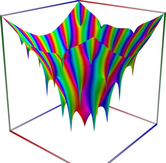
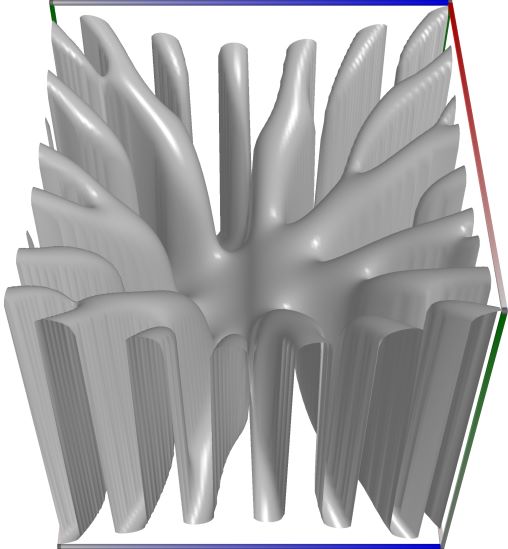
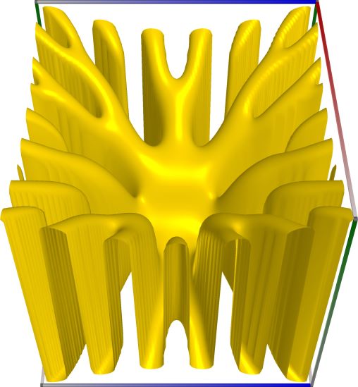
Left figure: real part of the Weierstrass Sigma function \(\sigma_g(z, g_2, g_3\)). Camera angles are \(\theta=135^\circ\) and \(\phi = -12^\circ\), camera radius is -2.
Middle figure: imaginary part of the Weierstrass Sigma function \(\sigma_g(z, g_2, g_3\)). Camera angles are \(\theta=135^\circ\) and \(\phi = -12^\circ\), camera radius is -2.
Right figure: absolute value of the Weierstrass Sigma function \(\sigma_g(z, g_2, g_3\)), with color-coded phase. Camera angles are \(\theta=135^\circ\) and \(\phi = -12^\circ\), camera radius is -2.
For \(\Delta = g_2^3 - 27 g_3^2 \ne 0\), we first compute the elliptic half periods \(\omega_1, \omega_2\) from the lattice invariants \(g_2, g_3\) (see EllipticHalfPeriodsG), and set \(\omega = \omega_1, \tau = \omega_2/\omega_1\). Then \(\sigma_g(z; g_2, g_3) = \sigma(z| \omega, \tau)\) (see WeierstrassSigma).
For \(\Delta = 0, g_2 > 0, g_3 \ne 0\), the function \(\sigma_g(\cdot)\) can be expressed in closed form in terms of elementary functions:
For \(\Delta = 0, g_2 > 0, g_3 < 0: \quad \displaystyle \sigma_g(z; g_2, g_3) = \frac{\sinh( \sqrt{3c}z )}{\sqrt{3c} \cdot e^{cx^2 /2}}, \quad \text{where } c = \sqrt{g_2/12}\).
For \(\Delta = 0, g_2 > 0, g_3 > 0: \quad \displaystyle \sigma_g(z; g_2, g_3) = \frac{\sin( \sqrt{3c}z )}{\sqrt{3c} \cdot e^{cx^2 /2}}, \quad \text{where } c = \sqrt{g_2/12}\).
If both \(g_2\) and \(g_3\) are zero, the function \(\sigma_g(\cdot)\) becomes \(\sigma_g(z; 0, 0) = z\).
An example with real input for \(z\) and with purely imaginary input for \(\tau\), producing real output:
>>> from xlcalcnet import dec, mpm, gmp, fpm, apm
>>> mpm.dps = 40; z = '0.1'; tau = '0.0 + 0.9j'
>>> \mathrm{d}x = dec.weierstrass_sigma(z, tau); mx = mpm.weierstrass_sigma(z, tau)
>>> gx = gmp.weierstrass_sigma(z, tau)
>>> fx = fpm.weierstrass_sigma(z, tau); ax = apm.weierstrass_sigma(z, tau)
>>> mpm.show([\mathrm{d}x, mx, gx, fx, ax])
dec:  9.998992989830383649264433694319757846077E-2
mpm:  9.998992989830383649264433694319757846077e-2
gmp:  9.998992989830383649264433694319757846077E-02
fpm:  9.99899298983038E-02
apm:  9.998992989830383649264433694319757846077e-2 (5.023e-39%)