Spirals#
Archimedes’ spiral#
- User.ArchimedesSpiral(a, Resolution, AsPolar=false)#
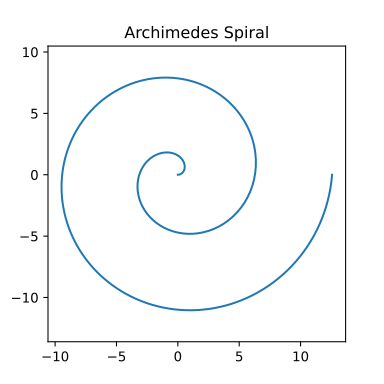
The parametric equations of Archimedes’ Spiral are
\[r(t) = a t,\]\[x(t) = r \cos(t),\]\[y(t) = r \sin(t).\]Changing the parameter \(a\) controls the distance between loops.
See also Wikipedia [1518], MathWorld [1146], MathCurve [316].
An example in Python
>>> from mpfunlab import User
>>> Curve = User.Cardioid(a = 1, Resolution = 200, AsPolar = true)
>>> User.Chart2D.Show(Curve, Template = 'PolarCurve', Title = 'Cardioid')
 \(\quad\) \(\quad\)
 Left figure: Archimedes Spiral
Middle figure: Archimedes Spiral
Right figure: Archimedes Spiral
Fermat’s spiral#
- User.FermatSpiral(a, Resolution, AsPolar=false)#
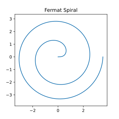
The parametric equations of Fermat’ spiral are
\[r(t) = \pm a \sqrt{t},\]\[x(t) = r \cos(t),\]\[y(t) = r \sin(t).\]Changing the parameter \(a\) controls the distance between loops.
See also Wikipedia [1529], MathWorld [1152], MathCurve [1529].
An example in Python
>>> from mpfunlab import User
>>> Curve = User.Cardioid(a = 1, Resolution = 200, AsPolar = true)
>>> User.Chart2D.Show(Curve, Template = 'PolarCurve', Title = 'Cardioid')
 \(\quad\) \(\quad\)
 Left figure: Fermat’s Spiral.
Middle figure: Fermat’s Spiral.
Right figure: Fermat’s Spiral.
Hyperbolic Spiral#
- User.HyperbolicSpiral(a, Resolution, AsPolar=false)#
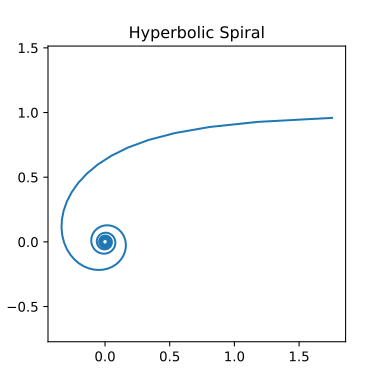
The parametric equations of the hyperbolic spiral are
\[r(t) = \frac{a}{t},\]\[x(t) = r \cos(t),\]\[y(t) = r \sin(t).\]Changing the parameter \(a\) controls the distance between loops.
See also Wikipedia [1533], MathWorld [1154], MathCurve [327].
An example in Python
>>> from mpfunlab import User
>>> Curve = User.Cardioid(a = 1, Resolution = 200, AsPolar = true)
>>> User.Chart2D.Show(Curve, Template = 'PolarCurve', Title = 'Cardioid')
 \(\quad\) \(\quad\)
 Left figure: Hyperbolic Spiral.
Middle figure: Hyperbolic Spiral.
Right figure: Hyperbolic Spiral.
Lituus#
- User.Lituus(a, Resolution, AsPolar=false)#
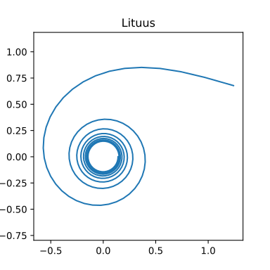
The parametric equations of the Lituus are
\[r(t) = \frac{a}{\sqrt{t}},\]\[x(t) = r \cos(t),\]\[y(t) = r \sin(t).\]Changing the parameter \(a\) controls the distance between loops.
See also Wikipedia [1537], MathWorld [1156], MathCurve [335].
An example in Python
>>> from mpfunlab import User
>>> Curve = User.Cardioid(a = 1, Resolution = 200, AsPolar = true)
>>> User.Chart2D.Show(Curve, Template = 'PolarCurve', Title = 'Cardioid')
 \(\quad\) \(\quad\)
 Left figure: Lituus.
Middle figure: Lituus.
Right figure: Lituus.
Logarithmic Spiral#
- User.LogarithmicSpiral(a, Resolution, AsPolar=false)#
The parametric equations of the logarithmic spiral are
\[r(t) = a \exp(k t),\]\[x(t) = r \cos(t),\]\[y(t) = r \sin(t).\]where \(a>0\) and \(k \ne 0\) are real constants.
See also Wikipedia [1538], MathWorld [1157], MathCurve [336].
An example in Python
>>> from mpfunlab import User
>>> Curve = User.Cardioid(a = 1, Resolution = 200, AsPolar = true)
>>> User.Chart2D.Show(Curve, Template = 'PolarCurve', Title = 'Cardioid')
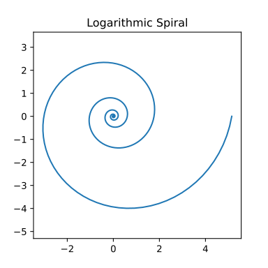 \(\quad\) \(\quad\)
 Left figure: Logarithmic Spiral.
Middle figure: Logarithmic Spiral.
Right figure: Logarithmic Spiral.
Poinsot’s Spiral#
- User.PoinsotSpiral(a, Resolution, AsPolar=false)#
The parametric equations of the Poinsot spiral are
\[r(t) = \frac{a}{\alpha \cosh(k t) + \beta \sinh(k t)}, \quad \text{with } \alpha^2 + \beta^2 \ne 0.\]\[x(t) = r \cos(t),\]\[y(t) = r \sin(t).\]where \(a>0\) and \(k \ne 0\) are real constants.
See also Wikipedia [1599], MathWorld [1169], MathCurve [346].
An example in Python
>>> from mpfunlab import User
>>> Curve = User.Cardioid(a = 1, Resolution = 200, AsPolar = true)
>>> User.Chart2D.Show(Curve, Template = 'PolarCurve', Title = 'Cardioid')
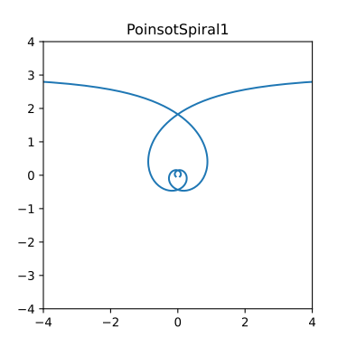 \(\quad\)
 Left figure: Poinsot’s Spiral, type 1.
Middle figure: Poinsot’s Spiral, type 2.
Cotes’s spiral#
- User.CotesSpiral(a, Resolution, AsPolar=false)#
The shape of spirals in the family depends on the parameters. The curves in polar coordinates, \((r, \theta), r>0\) are defined by one of the following five equations:
\[\begin{split}\frac{1}{r} = \begin{cases} A \cosh(k\theta + \varepsilon) \\ A \exp(k\theta + \varepsilon) \\ A \sinh(k\theta + \varepsilon) \\ A (k\theta + \varepsilon) \\ A \cos(k\theta + \varepsilon) \\ \end{cases}\end{split}\]\(A > 0\), \(k > 0\) and \(\varepsilon\) are arbitrary real constants. \(A\) determines the size, \(k\) determines the shape, and \(\varepsilon\) determines the angular position of the spiral.
The first and third forms are Poinsot’s spirals; the second is the logarithmic spiral; the fourth is the hyperbolic spiral; the fifth is the epispiral.
See also Wikipedia [1590], MathWorld [1164].
An example in Python
>>> from mpfunlab import User
>>> Curve = User.Cardioid(a = 1, Resolution = 200, AsPolar = true)
>>> User.Chart2D.Show(Curve, Template = 'PolarCurve', Title = 'Cardioid')
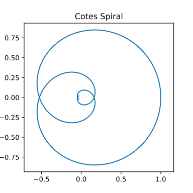 \(\quad\) \(\quad\)
 Left figure: Cote’s Spirals.
Middle figure: Cote’s Spirals.
Right figure: Cote’s Spirals.
Tanh Spiral#
- User.TanhSpiral(a, Resolution, AsPolar=false)#
This is a spiral proposed by Bourke [39], and also discussed by Meier [435]. It has the following parametric equations:
\[x(t) = \frac{\sinh(2t)}{\cos(2at) + \cosh(2t)},\]\[y(t) = \frac{\sin(2at)}{\cos(2at) + \cosh(2t)},\]with \(-\pi/2 \le t \le \pi/2\) and \(a>0\) (eg:2).
An example in Python
>>> from mpfunlab import User
>>> Curve = User.Cardioid(a = 1, Resolution = 200, AsPolar = true)
>>> User.Chart2D.Show(Curve, Template = 'PolarCurve', Title = 'Cardioid')
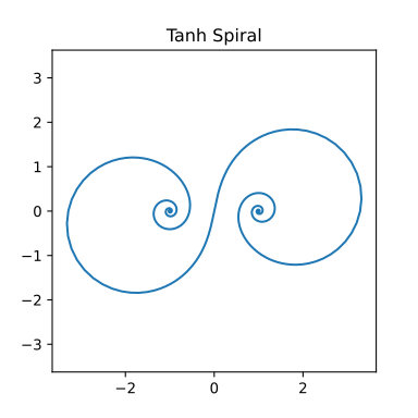 \(\quad\) \(\quad\)
 Left figure: Tanh Spiral.
Middle figure: Tanh Spiral.
Right figure: Tanh Spiral.
Nielsens Spiral#
- User.NielsenSpiral(a, Resolution, AsPolar=false)#
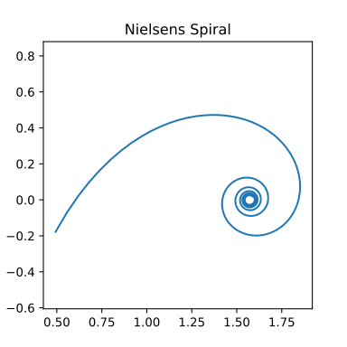
Nielsen’s spiral, also called the sici spiral is the spiral with parametric equations
\[x(t) = a \cdot \mathrm{ci}(t),\]\[y(t) = a \cdot \mathrm{si}(t),\]where \(\mathrm{ci}(t)\) is the cosine integral and \(\mathrm{si}(t)\) is the sine integral.
See also Wikipedia [1598], MathWorld [1168], MathCurve [349].
An example in Python
>>> from mpfunlab import User
>>> Curve = User.Cardioid(a = 1, Resolution = 200, AsPolar = true)
>>> User.Chart2D.Show(Curve, Template = 'PolarCurve', Title = 'Cardioid')
 \(\quad\) \(\quad\)
 Left figure: Nielsens Spiral.
Middle figure: Nielsens Spiral.
Right figure: Nielsens Spiral.
Cornu Spiral#
- User.CornuSpiral(a, Resolution, AsPolar=false)#
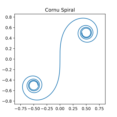
The Cornu spiral, also known as a Euler spiral or clothoid, is the curve generated by a parametric plot of S(t) against C(t). A Cornu spiral has the property that its curvature at any point is proportional to the distance along the spiral, measured from the origin.
\[x(t) = a \cdot C(t),\]\[y(t) = a \cdot S(t),\]where \(C(t)\) and \(S(t)\) are the Fresnel integrals.
See also Wikipedia [1593], MathWorld [1163], MathCurve [342].
An example in Python
>>> from mpfunlab import User
>>> Curve = User.Cardioid(a = 1, Resolution = 200, AsPolar = true)
>>> User.Chart2D.Show(Curve, Template = 'PolarCurve', Title = 'Cardioid')
 \(\quad\) \(\quad\)
 Left figure: Cornu Spiral.
Middle figure: Cornu Spiral.
Right figure: Cornu Spiral.