Miscellaneous functions

Lambert \(W\) function, \(W_0(x)\)

ctx.lambert_w0(x)

where ctx is math53, ctxboost or ctxflint.

Returns \(W_0(x)\), the real-valued principal branch of the Lambert W function for \(x > -1/e\), with \(W_0(x) \ge -1\) for \(x<0\). The Lambert W function is defined as the solution of \(x = W(x) \exp(W(x))\).

See also Wikipedia [1368], MathWorld [964], NIST [513], BoostMath [112], Corless et al. [192], Ehrhardt [309] (3.10.15), Flint [810], Flint [800], Mpmath [622].

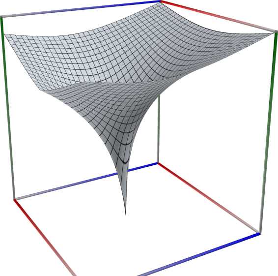\(\quad\) 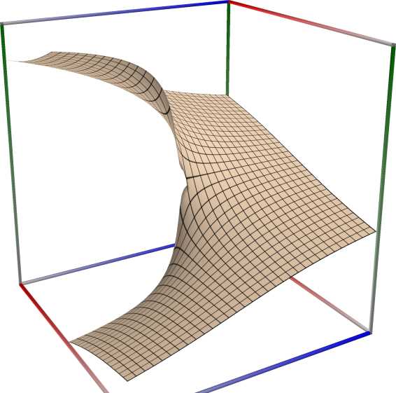\(\quad\)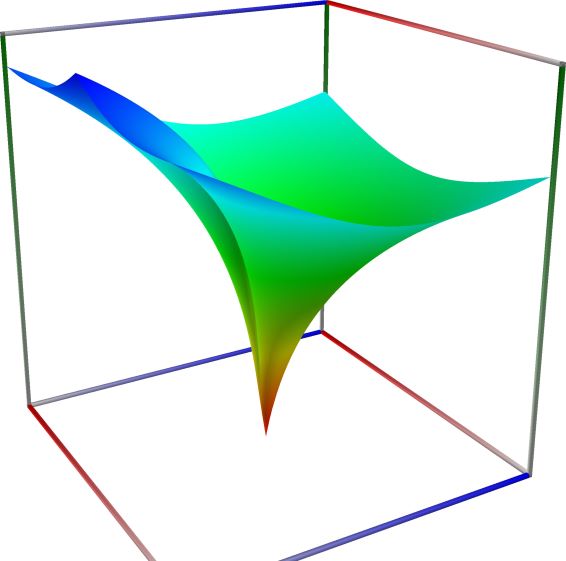

Left figure: real part of the LambertW function. Camera angles are \(\theta=135^\circ\) and \(\phi = -12^\circ\), camera radius is -2.

Middle figure: imaginary part of the LambertW function. Camera angles are \(\theta=135^\circ\) and \(\phi = -12^\circ\), camera radius is -2.

Right figure: absolute value of the LambertW function, with color-coded phase. Camera angles are \(\theta=135^\circ\) and \(\phi = -12^\circ\), camera radius is -2.

An example in Python

>>> from xlcalcnet import xreal
>>> xreal.LambertW(3.4)
xreal('5.2359877559829887307E-1')
>>> xreal.LambertW(13.4)
xreal('5.3518479027559984754E-1')

An example in Visual Basic

>>> from xlcalcnet import Gpr
>>> Gpr.LambertW(3.4)
Gpr('5.2359877559829887307E-1')
>>> Gpr.LambertW(13.4)
Gpr('5.3518479027559984754E-1')

Basic examples

The Lambert W function is the inverse of \(w \exp(w)\):

>>> from xlcalcnet import *
>>> mp.dps = 25; mp.pretty = True
>>> w = lambertw(1)
>>> w
0.5671432904097838729999687
>>> w*exp(w)
1.0

Any branch gives a valid inverse:

>>> w = lambertw(1, k=3)
>>> w
(-2.853581755409037807206819 + 17.11353553941214591260783j)
>>> w = lambertw(1, k=25)
>>> w
(-5.047020464221569709378686 + 155.4763860949415867162066j)
>>> chop(w*exp(w))
1.0

Lambert \(W\) function, \(W_{-1}(x)\)

ctx.lambert_wm1(x)

where ctx is math53, ctxboost or ctxflint.

Returns \(W_{-1}(x)\), the second real-valued, non-principal, branch of the Lambert W function for \(-1/e < x < 0\), with \(W_{-1}(x) \le -1\) for \(x<0\). The Lambert W function is defined as the solution of \(x = W(x) \exp(W(x))\), Flint [810], Flint [800].

See also Wikipedia [1368], MathWorld [964], NIST [513], BoostMath [112], Ehrhardt [309] (3.10.15), Mpmath [622].

An example in Python

>>> from xlcalcnet import xreal
>>> xreal.LambertW1(0.2)
xreal('5.2359877559829887307E-1')
>>> xreal.LambertW1(0.21)
xreal('5.3518479027559984754E-1')

An example in Visual Basic

>>> from xlcalcnet import Gpr
>>> Gpr.LambertW1(0.2)
Gpr('5.2359877559829887307E-1')
>>> Gpr.LambertW1(0.21)
Gpr('5.3518479027559984754E-1')

Basic examples

The Lambert W function is the inverse of \(w \exp(w)\):

>>> from xlcalcnet import *
>>> mp.dps = 25; mp.pretty = True
>>> w = lambertw(1)
>>> w
0.5671432904097838729999687
>>> w*exp(w)
1.0

Any branch gives a valid inverse:

>>> w = lambertw(1, k=3)
>>> w
(-2.853581755409037807206819 + 17.11353553941214591260783j)
>>> w = lambertw(1, k=25)
>>> w
(-5.047020464221569709378686 + 155.4763860949415867162066j)
>>> chop(w*exp(w))
1.0

Lambert \(W\) (general case)

ctx.lambert_wk(z, k=0)

where ctx is math53, ctxboost, ctxflint.

Returns the Lambertw function of z.

See also BoostMath [112], Wikipedia [1368], MathWorld [964], NIST [513], Corless et al. [192], Ehrhardt [309] (4.2.39), Flint [810], Flint [800], Mpmath [622].

The Lambert W function \(W(z)\) is defined as the inverse function of \(w \exp(w)\). In other words, the value of \(W(z)\) is such that \(z = W(z) \exp(W(z))\) for any complex number \(z\).

The Lambert W function is a multivalued function with infinitely many branches \(W_k(z)\), indexed by \(k \in \mathbb{Z}\). Each branch gives a different solution \(w\) of the equation \(z = w \exp(w)\). All branches are supported:

• lambertw(z) gives the principal solution (branch 0)

• lambertw(z, k) gives the solution on branch \(k\)

The Lambert W function has two partially real branches: the principal branch (\(k = 0\)) is real for real \(z > -1/e\), and the \(k = -1\) branch is real for \(-1/e < z < 0\). All branches except \(k = 0\) have a logarithmic singularity at \(z = 0\).

The definition, implementation and choice of branches is based on Corless et al. [192].

An example in Python

>>> from xlcalcnet import XComplex
>>> XComplex.LambertW(0.5, 2)
XComplex('5.2359877559829887307E-1')
>>> XComplex.LambertW('0.1')
XComplex('5.3518479027559984754E-1')

An example in Visual Basic

>>> from xlcalcnet import Gpc
>>> Gpc.LambertW(0.5, 2)
Gpc('5.2359877559829887307E-1')
>>> Gpc.LambertW('0.1')
Gpc('5.3518479027559984754E-1')

Basic examples

The Lambert W function is the inverse of \(w \exp(w)\):

>>> from xlcalcnet import *
>>> mp.dps = 25; mp.pretty = True
>>> w = lambertw(1)
>>> w
0.5671432904097838729999687
>>> w*exp(w)
1.0

Any branch gives a valid inverse:

>>> w = lambertw(1, k=3)
>>> w
(-2.853581755409037807206819 + 17.11353553941214591260783j)
>>> w = lambertw(1, k=25)
>>> w
(-5.047020464221569709378686 + 155.4763860949415867162066j)
>>> chop(w*exp(w))
1.0

Arithmetic-geometric mean

ctx.agm(x, y=1)

where ctx is math53, mathc53, ctxboost or ctxflint.

Returns the arithmetic-geometric mean of \(|x|\) and \(|y|\). See also Wikipedia [1378], MathWorld [986], Ehrhardt [309] (4.2.1), Ehrhardt [309] (4.2.2), Mpmath [630].

With \(a_0 = \max(|x|, |y|)\), \(b_0 = \min(|x|, |y|)\) the AGM is calculated using the recurrence formulas

\[a_{n+1} = \tfrac{1}{2} (a_n + b_n), \quad b_{n+1} = \sqrt{a_n b_n}.\]

The sequences converge quadratically to a common limit and \(a_n \geq b_n\). The iteration is terminated if \(a_n - b_n \leq \epsilon a_n\), where \(\epsilon\) is less than the square root of the machine epsilon. The result is \((a_n + b_n )/2\).

The function \(\text{agm}(a,b)\) can also be expressed in closed form in terms of the complete elliptic integral of the first kind \(K(k)\) as

\[\text{agm}(a,b) = \frac{(a+b)\pi}{4K((a-b)/(a+b))}.\]

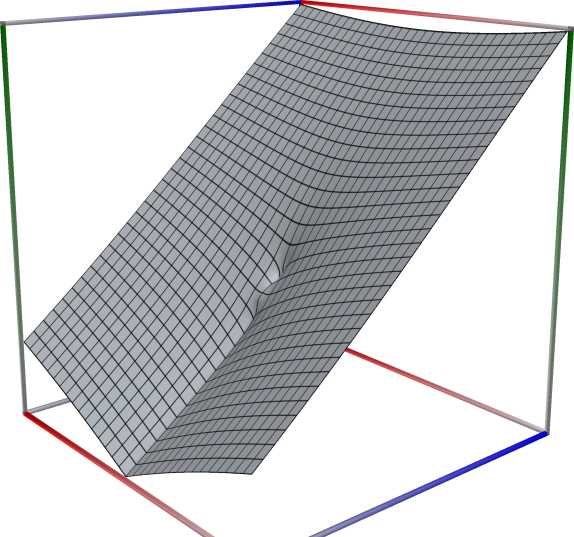\(\quad\) \(\quad\)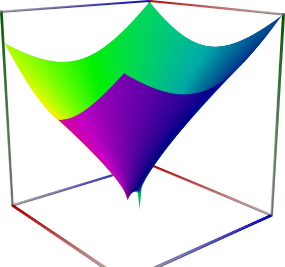

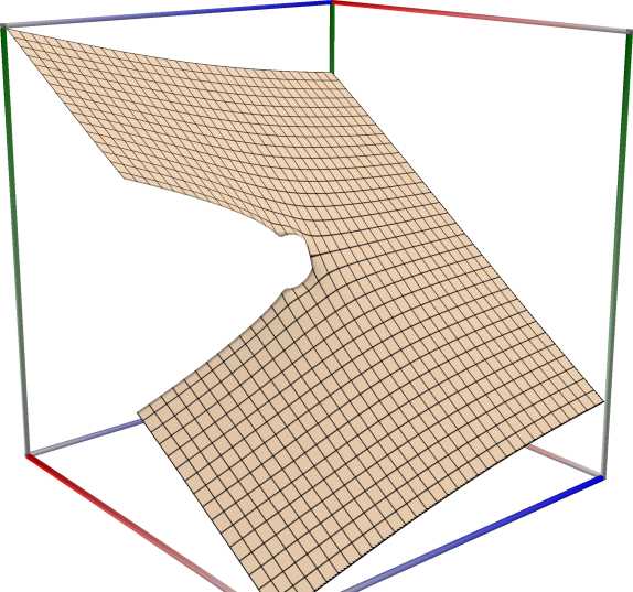
Left figure: real part of the AGM. Camera angles are \(\theta=135^\circ\) and \(\phi = -12^\circ\), camera radius is -2.

Middle figure: imaginary part of the AGM. Camera angles are \(\theta=135^\circ\) and \(\phi = -12^\circ\), camera radius is -2.

Right figure: absolute value of the AGM, with color-coded phase. Camera angles are \(\theta=135^\circ\) and \(\phi = -12^\circ\), camera radius is -2.

An example in Python

>>> from xlcalcnet import XComplex
>>> XComplex.Agm(0.5, 2)
XComplex('5.2359877559829887307E-1')
>>> XComplex.Agm('0.1')
XComplex('5.3518479027559984754E-1')

An example in Visual Basic

>>> from xlcalcnet import Gpc
>>> Gpc.Agm(0.5, 2)
Gpc('5.2359877559829887307E-1')
>>> Gpc.Agm('0.1')
Gpc('5.3518479027559984754E-1')

An example with real input:

>>> from xlcalcnet import dec, mpm, gmp, fpm, apm
>>> mpm.dps = 40; a = '0.6'; b = '0.3'
>>> \mathrm{d}x = dec.agm(a, b); mx = mpm.agm(a, b); gx = gmp.agm(a, b)
>>> fx = fpm.agm(a, b); ax = apm.agm(a, b)
>>> mpm.show([\mathrm{d}x, mx, gx, fx, ax])
dec:  4.370373093140720607559297149795245924922E-1
mpm:  4.370373093140720607559297149795245924922e-1
gmp:  4.370373093140720607559297149795245924922E-01
fpm:  4.37037309314072E-01
apm:  4.370373093140720607559297149795245924922e-1 (1.97e-39%)

An example with complex input:

>>> from xlcalcnet import dec, mpm, gmp, fpm, apm
>>> mpm.dps = 20; a = '5.0 + 2.0j'; b = '7.0 + 3.0j'
>>> \mathrm{d}z = dec.agm(a, b); mz = mpm.agm(a, b); gz = gmp.agm(a, b)
>>> fz = fpm.agm(a, b); az = apm.agm(a, b)
>>> mpm.show([\mathrm{d}z, mz, gz, fz, az], aligned=True)
dec: 5.9582264514273988109E+0              + 2.4753102663993183285E+0j
mpm: 5.9582264514273988109e+0              + 2.4753102663993183285e+0j
gmp: 5.9582264514273988109E+00             + 2.4753102663993183285E+00j
fpm: 5.95822645142740E+00                  + 2.47531026639932E+00j
apm: 5.9582264514273988109e+0 (1.137e-19%) + 2.4753102663993183285e+0 (1.369e-19%)j