Power functions#

Square, \(x^2\)#

ctx.sqr(x)#

where ctx is math53, mathc53, ctxcpp or ctxflint.

Returns the square function of \(x, x^2\). See also Wikipedia [1351], MathWorld [929], Ehrhardt [309] (4.1.18).

\(\quad\) \(\quad\)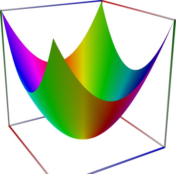

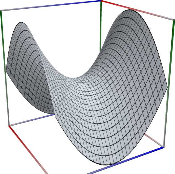
Left figure: real part of the Sqrt function. Camera angles are \(\theta=135^\circ\) and \(\phi = -12^\circ\), camera radius is -2.

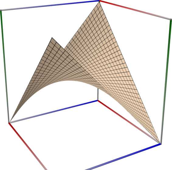
Middle figure: imaginary part of the Sqrt function. Camera angles are \(\theta=135^\circ\) and \(\phi = -12^\circ\), camera radius is -2.

Right figure: absolute value of the Sqrt function, with color-coded phase. Camera angles are \(\theta=135^\circ\) and \(\phi = -12^\circ\), camera radius is -2.

An example in Python

>>> from xlcalcnet import xreal
>>> xreal.Square(0.5)
xreal('5.2359877559829887307E-1')
>>> xreal.Square('0.51')
xreal('5.3518479027559984754E-1')

An example in Visual Basic

>>> from xlcalcnet import Gpr
>>> Gpr.Square(0.5)
Gpr('5.2359877559829887307E-1')
>>> Gpr.Square('0.51')
Gpr('5.3518479027559984754E-1')

Cube, \(x^3\)#

ctx.cube(x)#

where ctx is math53, mathc53, ctxcpp or ctxflint.

Returns the cube function of \(x, x^3\). See also Wikipedia [1351], MathWorld [929], Ehrhardt [309] (4.1.18).

\(\quad\) 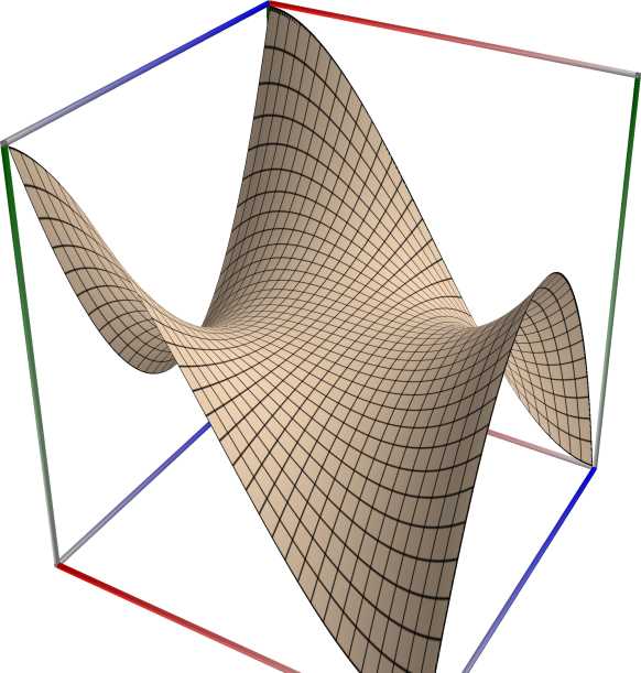\(\quad\)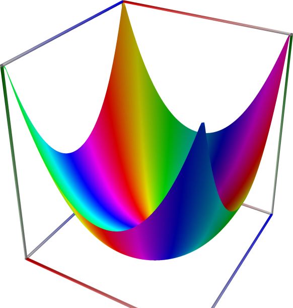

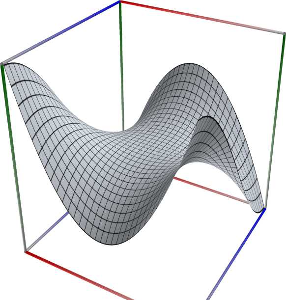
Left figure: real part of the Cube function. Camera angles are \(\theta=135^\circ\) and \(\phi = -12^\circ\), camera radius is -2.

Middle figure: imaginary part of the Cube function. Camera angles are \(\theta=135^\circ\) and \(\phi = -12^\circ\), camera radius is -2.

Right figure: absolute value of the Cube function, with color-coded phase. Camera angles are \(\theta=135^\circ\) and \(\phi = -12^\circ\), camera radius is -2.

An example in Python

>>> from xlcalcnet import xreal
>>> xreal.Square(0.5)
xreal('5.2359877559829887307E-1')
>>> xreal.Square('0.51')
xreal('5.3518479027559984754E-1')

An example in Visual Basic

>>> from xlcalcnet import Gpr
>>> Gpr.Square(0.5)
Gpr('5.2359877559829887307E-1')
>>> Gpr.Square('0.51')
Gpr('5.3518479027559984754E-1')

Auxiliary function \(\mathrm{powi}(x,n) = x^n\)#

ctx.powi(x, n)#

where ctx is math53, mathc53, ctxcpp or ctxflint.

Note: math53.intpower(x, n)

Returns the integer power function of \(x, x^n\). See also Wikipedia [1351], MathWorld [929].

An example in Python

>>> from xlcalcnet import xreal
>>> xreal.Intpower(0.5, 2)
xreal('5.2359877559829887307E-1')
>>> xreal.Intpower('0.51', 2)
xreal('5.3518479027559984754E-1')

An example in Visual Basic

>>> from xlcalcnet import Gpr
>>> Gpr.Intpower(0.5, 2)
Gpr('5.2359877559829887307E-1')
>>> Gpr.Intpower('0.51', 2)
Gpr('5.3518479027559984754E-1')

An example with real input:

>>> from xlcalcnet import dec, mpm, ipm
>>> mpm.dps = 40; x = '10.5'
>>> \mathrm{d}x = dec.square(x); mx = mpm.square(x); ix = ipm.square(x)
>>> mpm.show([\mathrm{d}x, mx, ix])
dec:  1.102500000000000000000000000000000000000E+2
mpm:  1.102500000000000000000000000000000000000e+2
ipm:  1.102500000000000000000000000000000000000e+2 (0.0%)

>>> from xlcalcnet import mpm, fpm, gmp, apm
>>> mpm.dps = 40; x = '10.5'
>>> fx = fpm.square(x); gx = gmp.square(x); ax = apm.square(x)
>>> mpm.show([fx, gx, ax])
fpm:  1.10250000000000E+02
gmp:  1.102500000000000000000000000000000000000E+02
apm:  1.102500000000000000000000000000000000000e+2 (0.0%)

The following example with complex input shows that the relative error can be high in double precision:

>>> from xlcalcnet import dec, mpm, ipm
>>> mpm.dps = 20; z = '10.2 + 1.5E-2j'
>>> \mathrm{d}z = dec.square(z); mz = mpm.square(z); iz = ipm.square(z)
>>> mpm.show([\mathrm{d}z, mz, iz], aligned=True)
dec: 1.0403977500000000000E+2              + 3.0600000000000000000E-1j
mpm: 1.0403977500000000000e+2              + 3.0600000000000000000e-1j
ipm: 1.0403977500000000000e+2 (2.084e-19%) + 3.0600000000000000000e-1 (2.076e-19%)j

>>> from xlcalcnet import mpm, fpm, gmp, apm
>>> mpm.dps = 20; z = '10.2 + 1.5E-2j'
>>> fz = fpm.square(z); gz = gmp.square(z); az = apm.square(z)
>>> mpm.show([fz, gz, az], aligned=True)
fpm: 1.04039775000000E+02                  + 3.06000000000000E-01j
gmp: 1.0403977500000000000E+02             + 3.0600000000000000000E-01j
apm: 1.0403977500000000000e+2 (2.084e-19%) + 3.0600000000000000000e-1 (2.076e-19%)j

Auxiliary function \(\mathrm{compound}(x,n) = (1+x)^n\)#

math53.compound(a, b)#

Returns \((1+x)^n\), computed accurately also when \(x\) is very close to 0.

An example in Python

>>> from xlcalcnet import xreal
>>> xreal.Compound(0.5, 2)
xreal('5.2359877559829887307E-1')
>>> xreal.Compound('0.51', 2)
xreal('5.3518479027559984754E-1')

An example in Visual Basic

>>> from xlcalcnet import Gpr
>>> Gpr.Compound(0.5, 2)
Gpr('5.2359877559829887307E-1')
>>> Gpr.Compound('0.51', 2)
Gpr('5.3518479027559984754E-1')

Auxiliary function \(\mathrm{comprel}(x,n) = (1+x)^n - 1\)#

math53.comprel(x, n)#

Returns \((1+x)^n - 1\), computed accurately also when \(x\) is very close to 0.

An example in Python

>>> from xlcalcnet import xreal
>>> xreal.Comprel(0.5, 2)
xreal('5.2359877559829887307E-1')
>>> xreal.Comprel('0.51', 2)
xreal('5.3518479027559984754E-1')

An example in Visual Basic

>>> from xlcalcnet import Gpr
>>> Gpr.Comprel(0.5, 2)
Gpr('5.2359877559829887307E-1')
>>> Gpr.Comprel('0.51', 2)
Gpr('5.3518479027559984754E-1')

Auxiliary function \(\mathrm{hypot}(x,y) = \sqrt{x^2 + y^2}\)#

ctx.hypot(x, y)#

where ctx is math53, mathc53, ctxcpp or ctxflint.

Returns \(\mathrm{hypot}(x, y) = \sqrt { x^2 + y^2 }\) in a way which avoids undue underflow and overflow. See also Wikipedia [1392], BoostMath [128], Mpmath [643].

The function is even and symmetric in \(x\) and \(y\), so we assume \(x,y > 0\) and \(x > y\) (we can permute the arguments if this is not the case). Then the result is calculated as:

\[\mathrm{hypot}(x, y) = x \sqrt {1 + \left( \frac{y}{x} \right)^2 }\]

An example in Python

>>> from xlcalcnet import xreal
>>> xreal.Hypot(0.5, 2)
xreal('5.2359877559829887307E-1')
>>> xreal.Hypot(0.5, 2)
xreal('5.3518479027559984754E-1')

An example in Visual Basic

>>> from xlcalcnet import Gpr
>>> Gpr.Hypot(0.5, 2)
Gpr('5.2359877559829887307E-1')
>>> Gpr.Hypot(0.5, 2)
Gpr('5.3518479027559984754E-1')

An example with real input:

>>> from xlcalcnet import dec, mpm, ipm
>>> mpm.dps = 40; a = '20.4'; b = '10.4'
>>> \mathrm{d}x = dec.hypot(a, b); mx = mpm.hypot(a, b); ix = ipm.hypot(a, b)
>>> mpm.show([\mathrm{d}x, mx, ix])
dec:  2.289803485017873755441437047351340654358E+1
mpm:  2.289803485017873755441437047351340654358e+1
ipm:  2.289803485017873755441437047351340654358e+1 (2.406e-39%)

>>> from xlcalcnet import mpm, fpm, gmp, apm
>>> mpm.dps = 40; a = '20.4'; b = '10.4'
>>> fx = fpm.hypot(a, b); gx = gmp.hypot(a, b); ax = apm.hypot(a, b)
>>> mpm.show([fx, gx, ax])
fpm:  2.28980348501787E+01
gmp:  2.289803485017873755441437047351340654358E+01
apm:  2.289803485017873755441437047351340654358e+1 (2.326e-38%)

The following example with complex input shows that the relative error can be high in double precision:

>>> from xlcalcnet import dec, mpm, ipm
>>> mpm.dps = 20; a = '20.2 + 1.5E+2j'; b = '10.7 + 2.3E+1j'
>>> \mathrm{d}z = dec.hypot(a, b); mz = mpm.hypot(a, b); iz = ipm.hypot(a, b)
>>> mpm.show([\mathrm{d}z, mz, iz], aligned=True)
dec: 2.1614348471624799140E+1              + 1.5157061080517169075E+2j
mpm: 2.1614348471624799140e+1              + 1.5157061080517169075e+2j
ipm: 2.1614348471624799140e+1 (3.762e-19%) + 1.5157061080517169075e+2 (1.431e-19%)j

>>> from xlcalcnet import mpm, fpm, gmp, apm
>>> mpm.dps = 20; a = '20.2 + 1.5E+2j'; b = '10.7 + 2.3E+1j'
>>> fz = fpm.hypot(a, b); gz = gmp.hypot(a, b); az = apm.hypot(a, b)
>>> mpm.show([fz, gz, az], aligned=True)
fpm: 2.16143484716248E+01                  + 1.51570610805172E+02j
gmp: 2.1614348471624799140E+01             + 1.5157061080517169075E+02j
apm: 2.1614348471624799140e+1 (2.508e-18%) + 1.5157061080517169075e+2 (3.29e-18%)j

Power function, \(\mathrm{pow}(x, y) = x^y\)#

ctx.pow(x, y)#

where ctx is math53, mathc53, ctxcpp, ctxflint.

Returns \(x^{y} = \exp(y \log(x))\). See also Wikipedia [1356], Wikipedia [1343], MathWorld [926], NIST [514], Ehrhardt [309] (4.2.34), Flint [811], Flint [801], Mpmath [582].

An example in Python

>>> from xlcalcnet import xreal
>>> xreal.Pow(0.5, 3)
xreal('5.2359877559829887307E-1')
>>> xreal.Pow('0.51', 3)
xreal('5.3518479027559984754E-1')

An example in Visual Basic

>>> from xlcalcnet import Gpr
>>> Gpr.Pow(0.5, 3)
Gpr('5.2359877559829887307E-1')
>>> Gpr.Pow('0.51', 3)
Gpr('5.3518479027559984754E-1')

An example with real input:

>>> from xlcalcnet import dec, mpm, ipm
>>> mpm.dps = 40; a = '20.4'; b = '10.4'
>>> \mathrm{d}x = dec.power(a, b); mx = mpm.power(a, b); ix = ipm.power(a, b)
>>> mpm.show([\mathrm{d}x, mx, ix])
dec:  4.170169822990247098901482655229494083311E+13
mpm:  4.170169822990247098901482655229494083310e+13
ipm:  4.170169822990247098901482655229494083312e+13 (3.874e-38%)

>>> from xlcalcnet import mpm, fpm, gmp, apm
>>> mpm.dps = 40; a = '20.4'; b = '10.4'
>>> fx = fpm.power(a, b); gx = gmp.power(a, b); ax = apm.power(a, b)
>>> mpm.show([fx, gx, ax])
fpm:  4.17016982299025E+13
gmp:  4.170169822990247098901482655229494083310E+13
apm:  4.170169822990247098901482655229494083312e+13 (3.874e-38%)

The following example with complex input shows that the relative error can be high in double precision:

>>> from xlcalcnet import dec, mpm, ipm
>>> mpm.dps = 20; a = '20.2 + 1.5E+2j'; b = '10.7 + 2.3E+1j'
>>> \mathrm{d}z = dec.power(a, b); mz = mpm.power(a, b); iz = ipm.power(a, b)
>>> mpm.show([\mathrm{d}z, mz, iz], aligned=True)
dec: 4.0882536339987303539E+8              - 8.4545584653874710182E+8j
mpm: 4.0882536339987303540e+8              - 8.4545584653874710183e+8j
ipm: 4.0882536339987303538e+8 (5.951e-18%) - 8.4545584653874710180e+8 (-4.195e-18%)j

>>> from xlcalcnet import mpm, fpm, gmp, apm
>>> mpm.dps = 20; a = '20.2 + 1.5E+2j'; b = '10.7 + 2.3E+1j'
>>> fz = fpm.power(a, b); gz = gmp.power(a, b); az = apm.power(a, b)
>>> mpm.show([fz, gz, az], aligned=True)
fpm: 4.08825363399861E+08                  - 8.45455846538744E+08j
gmp: 4.0882536339987303540E+08             - 8.4545584653874710183E+08j
apm: 4.0882536339987303538e+8 (5.951e-18%) - 8.4545584653874710180e+8 (-4.195e-18%)j

Auxiliary function, \(\mathrm{powm1}(x, y) = x^y-1\)#

ctx.powm1(a, b)#

where ctx is math53, mathc53, ctxcpp or ctxflint.

Returns \(a^b - 1\), computed accurately also when \(a^b\) is very close to 1. This is calculated as \(\mathrm{powm1}(a, b) = \mathrm{expm1}( b \mathrm{log}(a))\). See also Wikipedia [1343], MathWorld [926], NIST [514], BoostMath [97], Mpmath [647].

An example in Python

>>> from xlcalcnet import xreal
>>> xreal.Powm1(0.5, 3)
xreal('5.2359877559829887307E-1')
>>> xreal.Powm1(0.5, 3)
xreal('5.3518479027559984754E-1')

An example in Visual Basic

>>> from xlcalcnet import Gpr
>>> Gpr.Powm1(0.5, 3)
Gpr('5.2359877559829887307E-1')
>>> Gpr.Powm1(0.5, 3)
Gpr('5.3518479027559984754E-1')

From mpmath:

>>> from xlcalcnet import mp
>>> mp.dps = 15; mp.pretty = True
>>> power(0.99999995, 1e-10) - 1
0.0
>>> powm1(0.99999995, 1e-10)
-5.00000012791934e-18

An example with real input:

>>> from xlcalcnet import dec, mpm, ipm
>>> mpm.dps = 40; a = '0.99999995'; b = '1e-10'
>>> \mathrm{d}x = dec.powm1(a, b); mx = mpm.powm1(a, b); ix = ipm.powm1(a, b)
>>> mpm.show([\mathrm{d}x, mx, ix])
dec:  -5.000000125000004154166822291672888041926E-18
mpm:  -5.000000125000004154166822291672887919513e-18
ipm:  -5.000000125000004154166822291672888493485e-18 (-1.148e-32%)

>>> from xlcalcnet import mpm, fpm, gmp, apm
>>> mpm.dps = 40; a = '0.99999995'; b = '1e-10'
>>> fx = fpm.powm1(a, b); gx = gmp.powm1(a, b); ax = apm.powm1(a, b)
>>> mpm.show([fx, gx, ax])
fpm:  -5.00000012791934E-18
gmp:  -5.000000125000004154166822291672887919513E-18
apm:  -5.000000125000004154166822291672888045069e-18 (-1.168e-32%)

The following example with complex input shows that the relative error can be high in double precision:

>>> from xlcalcnet import dec, mpm, ipm
>>> mpm.dps = 20; a = '0.99999995 + 1.5E-12j'; b = '1e-10 + 2.3E-10j'
>>> \mathrm{d}z = dec.powm1(a, b); mz = mpm.powm1(a, b); iz = ipm.powm1(a, b)
>>> mpm.show([\mathrm{d}z, mz, iz], aligned=True)
dec: -5.0003451250172541087E-18              - 1.1499850287492509267E-17j
mpm: -5.0003451250172909401e-18              - 1.1499850287492593979e-17j
ipm: -5.0003451250172485884e-18 (-8.47e-13%) - 1.1499850287492496570e-17 (-8.47e-13%)j

>>> from xlcalcnet import mpm, fpm, gmp, apm
>>> mpm.dps = 20; a = '0.99999995 + 1.5E-12j'; b = '1e-10 + 2.3E-10j'
>>> fz = fpm.powm1(a, b); gz = gmp.powm1(a, b); az = apm.powm1(a, b)
>>> mpm.show([fz, gz, az], aligned=True)
fpm: -5.00034512793659E-18                    - 1.14998502942070E-17j
gmp: -5.0003451250172909401E-18               - 1.1499850287492593979E-17j
apm: -5.0003451250172552059e-18 (-8.899e-13%) - 1.1499850287492511790e-17 (-8.783e-13%)j

Auxiliary function, \(\mathrm{pow1p}(x, y) = (1+x)^y\)#

ctx.pow1p(x, y)#

where ctx is math53, mathc53, ctxcpp or ctxflint.

Returns \((1+x)^y, x > -1\), with dbl2 arithmetic for critical values.

Returns \((1+x)^y\). This is calculated as \(\mathrm{pow1p}(x, y) = \mathrm{exp}(y \mathrm{logp1}(x))\).

An example in Python

>>> from xlcalcnet import xreal
>>> xreal.Pow1p(0.5, 3)
xreal('5.2359877559829887307E-1')
>>> xreal.Pow1p(0.5, 3)
xreal('5.3518479027559984754E-1')

An example in Visual Basic

>>> from xlcalcnet import Gpr
>>> Gpr.Pow1p(0.5, 3)
Gpr('5.2359877559829887307E-1')
>>> Gpr.Pow1p(0.5, 3)
Gpr('5.3518479027559984754E-1')

An example with real input:

>>> from xlcalcnet import dec, mpm, ipm
>>> mpm.dps = 40; a = '0.000005'; b = '1e-5'
>>> \mathrm{d}x = dec.pow1p(a, b); mx = mpm.pow1p(a, b); ix = ipm.pow1p(a, b)
>>> mpm.show([\mathrm{d}x, mx, ix])
dec:  1.000000000049999875001666658854222395521E+0
mpm:  1.000000000049999875001666658854222395521e+0
ipm:  1.000000000049999875001666658854222395521e+0 (1.148e-39%)

>>> from xlcalcnet import mpm, fpm, gmp, apm
>>> mpm.dps = 40; a = '0.000005'; b = '1e-5'
>>> fx = fpm.pow1p(a, b); gx = gmp.pow1p(a, b); ax = apm.pow1p(a, b)
>>> mpm.show([fx, gx, ax])
fpm:  1.00000000005000E+00
gmp:  1.000000000049999875001666658854222395521E+00
apm:  1.000000000049999875001666658854222395521e+0 (4.592e-39%)

The following example with complex input shows that the relative error can be high in double precision:

>>> from xlcalcnet import dec, mpm, ipm
>>> mpm.dps = 20; a = '0.000005 + 1.5E-12j'; b = '1e-5 + 2.3E-10j'
>>> \mathrm{d}z = dec.pow1p(a, b); mz = mpm.pow1p(a, b); iz = ipm.pow1p(a, b)
>>> mpm.show([\mathrm{d}z, mz, iz], aligned=True)
dec: 1.0000000000499998750E+0             + 1.1649970500682080027E-15j
mpm: 1.0000000000499998750e+0             + 1.1649970500682080027e-15j
ipm: 1.0000000000499998750e+0 (8.47e-20%) + 1.1649970500682080026e-15 (1.653e-17%)j

>>> from xlcalcnet import mpm, fpm, gmp, apm
>>> mpm.dps = 20; a = '0.000005 + 1.5E-12j'; b = '1e-5 + 2.3E-10j'
>>> fz = fpm.pow1p(a, b); gz = gmp.pow1p(a, b); az = apm.pow1p(a, b)
>>> mpm.show([fz, gz, az], aligned=True)
fpm: 1.00000000005000E+00                  + 1.16499705006821E-15j
gmp: 1.0000000000499998750E+00             + 1.1649970500682080027E-15j
apm: 1.0000000000499998750e+0 (1.694e-19%) + 1.1649970500682080027e-15 (5.166e-19%)j

Auxiliary function, \(\mathrm{pow1pm1}(x, y) = (1+x)^y - 1\)#

ctx.pow1pm1(x, y)#

where ctx is math53, mathc53, ctxcpp or ctxflint.

Returns \((1+x)^y - 1, x > -1\), special code for small \(x, y\).

This is calculated as \(\mathrm{pow1pm1}(x, y) = \mathrm{expm1}( y \cdot \mathrm{logp1}(x))\).

An example in Python

>>> from xlcalcnet import xreal
>>> xreal.Sqrt(0.5)
xreal('5.2359877559829887307E-1')
>>> xreal.Sqrt('0.51')
xreal('5.3518479027559984754E-1')

An example in Visual Basic

>>> from xlcalcnet import Gpr
>>> Gpr.Sqrt(0.5)
Gpr('5.2359877559829887307E-1')
>>> Gpr.Sqrt('0.51')
Gpr('5.3518479027559984754E-1')

An example with real input:

>>> from xlcalcnet import dec, mpm, ipm
>>> mpm.dps = 40; a = '0.000005'; b = '1e-5'
>>> \mathrm{d}x = dec.pow1pm1(a, b); mx = mpm.pow1pm1(a, b); ix = ipm.pow1pm1(a, b)
>>> mpm.show([\mathrm{d}x, mx, ix])
dec:  4.999987500166665885422239552083521142282E-11
mpm:  4.999987500166665885422239552083521142282e-11
ipm:  4.999987500166665885422239552083521142275e-11 (2.272e-37%)

>>> from xlcalcnet import mpm, fpm, gmp, apm
>>> mpm.dps = 40; a = '0.000005'; b = '1e-5'
>>> fx = fpm.pow1pm1(a, b); gx = gmp.pow1pm1(a, b); ax = apm.pow1pm1(a, b)
>>> mpm.show([fx, gx, ax])
fpm:  4.99998750016667E-11
gmp:  4.999987500166665885422239552083521142282E-11
apm:  4.999987500166665885422239552083521142282e-11 (5.346e-39%)

The following example with complex input shows that the relative error can be high in double precision:

>>> from xlcalcnet import dec, mpm, ipm
>>> mpm.dps = 20; a = '0.000005 + 1.5E-12j'; b = '1e-5 + 2.3E-10j'
>>> \mathrm{d}z = dec.pow1pm1(a, b); mz = mpm.pow1pm1(a, b); iz = ipm.pow1pm1(a, b)
>>> mpm.show([\mathrm{d}z, mz, iz], aligned=True)
dec: 4.9999875001321660590E-11              + 1.1649970500682080027E-15j
mpm: 4.9999875001321660590e-11              + 1.1649970500682080027e-15j
ipm: 4.9999875001321660585e-11 (1.676e-17%) + 1.1649970500682080026e-15 (1.653e-17%)j

>>> from xlcalcnet import mpm, fpm, gmp, apm
>>> mpm.dps = 20; a = '0.000005 + 1.5E-12j'; b = '1e-5 + 2.3E-10j'
>>> fz = fpm.pow1pm1(a, b); gz = gmp.pow1pm1(a, b); az = apm.pow1pm1(a, b)
>>> mpm.show([fz, gz, az], aligned=True)
fpm: 4.99998750013217E-11                   + 1.16499705006821E-15j
gmp: 4.9999875001321660590E-11              + 1.1649970500682080027E-15j
apm: 4.9999875001321660589e-11 (3.944e-19%) + 1.1649970500682080027e-15 (5.166e-19%)j

Power functions

Contents

Power functions#

Square, \(x^2\)#

Cube, \(x^3\)#

Auxiliary function \(\mathrm{powi}(x,n) = x^n\)#

Auxiliary function \(\mathrm{compound}(x,n) = (1+x)^n\)#

Auxiliary function \(\mathrm{comprel}(x,n) = (1+x)^n - 1\)#

Auxiliary function \(\mathrm{hypot}(x,y) = \sqrt{x^2 + y^2}\)#

Power function, \(\mathrm{pow}(x, y) = x^y\)#

Auxiliary function, \(\mathrm{powm1}(x, y) = x^y-1\)#

Auxiliary function, \(\mathrm{pow1p}(x, y) = (1+x)^y\)#

Auxiliary function, \(\mathrm{pow1pm1}(x, y) = (1+x)^y - 1\)#