Inverse hyperbolic functions#
For a general introduction to inverse hyperbolic functions, see Wikipedia [1367], NIST [511].
Inverse hyperbolic sine, \(\mathrm{asinh}(x)\)#
- ctx.asinh(x)#
where
ctxismath53,mathc53,ctxcpporctxflint.Returns the inverse hyperbolic sine of \(x\), \(\mathrm{asinh}(x)\). See also Wikipedia [1367], MathWorld [962], NIST [511], Ehrhardt [309] (4.2.14), Flint [808], Flint [798], Mpmath [601].
The inverse hyperbolic sine can be defined as \(\displaystyle \mathrm{asinh}(x) = \log \left(x+\sqrt{1+x^2}\right)\). The domain is the whole real line.
The inverse hyperbolic sine can be expressed in terms of related functions (with the principal-branch log and square root):
\[\mathrm{asinh}(z) = \log \left(z+\sqrt{1+z^2}\right) = \frac{1}{i} \mathrm{asin}(iz)\]
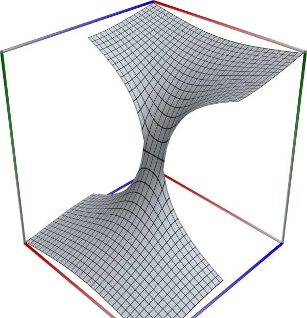 \(\quad\)
 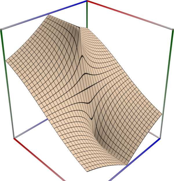 \(\quad\)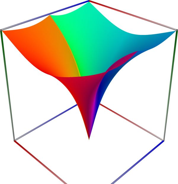
Left figure: real part of the Inverse Hyperbolic Sine function. Camera angles are \(\theta=135^\circ\) and \(\phi = -12^\circ\), camera radius is -2.
Middle figure: imaginary part of the Inverse Hyperbolic Sine function. Camera angles are \(\theta=135^\circ\) and \(\phi = -12^\circ\), camera radius is -2.
Right figure: absolute value of the Inverse Hyperbolic Sine function, with color-coded phase. Camera angles are \(\theta=135^\circ\) and \(\phi = -12^\circ\), camera radius is -2.
An example in Python
>>> from xlcalcnet import xreal
>>> xreal.Asinh(0.5)
xreal('5.2359877559829887307E-1')
>>> xreal.Asinh('0.51')
xreal('5.3518479027559984754E-1')
An example in Visual Basic
>>> from xlcalcnet import Gpr
>>> Gpr.Asinh(0.5)
Gpr('5.2359877559829887307E-1')
>>> Gpr.Asinh('0.51')
Gpr('5.3518479027559984754E-1')
An example with real input:
>>> from xlcalcnet import dec, mpm, ipm
>>> mpm.dps = 40; x = '1'
>>> \mathrm{d}x = dec.asinh(x); mx = mpm.asinh(x); ix = ipm.asinh(x)
>>> mpm.show([\mathrm{d}x, mx, ix])
dec:  8.813735870195430252326093249797923090282E-1
mpm:  8.813735870195430252326093249797923090282e-1
ipm:  8.813735870195430252326093249797923090282e-1 (3.907e-39%)

>>> from xlcalcnet import mpm, fpm, gmp, apm
>>> mpm.dps = 40; x = '1'
>>> fx = fpm.asinh(x); gx = gmp.asinh(x); ax = apm.asinh(x)
>>> mpm.show([fx, gx, ax])
fpm:  8.81373587019543E-01
gmp:  8.813735870195430252326093249797923090282E-01
apm:  8.813735870195430252326093249797923090282e-1 (6.512e-40%)
The following example with complex input shows that the relative error can be high in double precision:
>>> from xlcalcnet import dec, mpm, ipm
>>> mpm.dps = 20; z = '1 + 1.5E+2j'
>>> \mathrm{d}z = dec.asinh(z); mz = mpm.asinh(z); iz = ipm.asinh(z)
>>> mpm.show([\mathrm{d}z, mz, iz], aligned=True)
dec: 5.7037935865697639286E+0              + 1.5641296107511107312E+0j
mpm: 5.7037935865697639286e+0              + 1.5641296107511107312e+0j
ipm: 5.7037935865697639120e+0 (5.704e-16%) + 1.5641296107511107313e+0 (3.016e-17%)j

>>> from xlcalcnet import mpm, fpm, gmp, apm
>>> mpm.dps = 20; z = '1 + 1.5E+2j'
>>> fz = fpm.asinh(z); gz = gmp.asinh(z); az = apm.asinh(z)
>>> mpm.show([fz, gz, az], aligned=True)
fpm: 5.70379358656976E+00                  + 1.56412961075111E+00j
gmp: 5.7037935865697639286E+00             + 1.5641296107511107312E+00j
apm: 5.7037935865697639283e+0 (1.936e-17%) + 1.5641296107511107312e+0 (1.083e-18%)j
Inverse hyperbolic cosine, \(\mathrm{acosh}(x)\)#
- ctx.acosh(x)#
where
ctxismath53,mathc53,ctxcpporctxflint.Returns the inverse hyperbolic cosine of \(x\), \(\mathrm{acosh}(x)\). See also Wikipedia [1367], MathWorld [959], NIST [511], Ehrhardt [309] (4.2.4), Flint [808], Flint [798], Mpmath [598].
The inverse hyperbolic cosine can be defined as \(\displaystyle \mathrm{acosh}(x) = \log \left(x+\sqrt{x^2-1}\right)\). The domain is the closed interval \([1, +\infty)\).
The inverse hyperbolic cosine can be expressed in terms of related functions (with the principal-branch log and square root):
\[\mathrm{acosh}(z) = \log\left(z+\sqrt{z+1}\sqrt{z-1}\right) = \frac{\sqrt{z-1}}{\sqrt{1-z}} \mathrm{acos}(z)\]
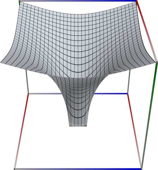 \(\quad\)
 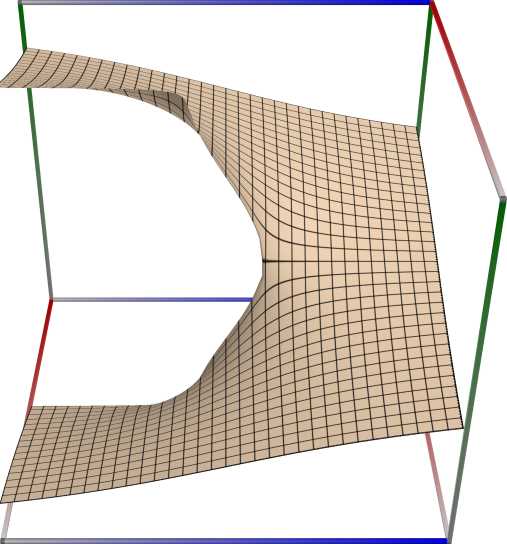 \(\quad\)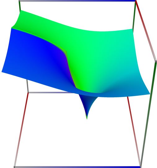
Left figure: real part of the Inverse Hyperbolic Cosine function. Camera angles are \(\theta=135^\circ\) and \(\phi = -12^\circ\), camera radius is -2.
Middle figure: imaginary part of the Inverse Hyperbolic Cosine function. Camera angles are \(\theta=135^\circ\) and \(\phi = -12^\circ\), camera radius is -2.
Right figure: absolute value of the Inverse Hyperbolic Cosine function, with color-coded phase. Camera angles are \(\theta=135^\circ\) and \(\phi = -12^\circ\), camera radius is -2.
An example in Python
>>> from xlcalcnet import xreal
>>> xreal.Acosh(0.5)
xreal('5.2359877559829887307E-1')
>>> xreal.Acosh('0.51')
xreal('5.3518479027559984754E-1')
An example in Visual Basic
>>> from xlcalcnet import Gpr
>>> Gpr.Acosh(0.5)
Gpr('5.2359877559829887307E-1')
>>> Gpr.Acosh('0.51')
Gpr('5.3518479027559984754E-1')
An example with real input:
>>> from xlcalcnet import dec, mpm, ipm
>>> mpm.dps = 40; x = '2'
>>> \mathrm{d}x = dec.acosh(x); mx = mpm.acosh(x); ix = ipm.acosh(x)
>>> mpm.show([\mathrm{d}x, mx, ix])
dec:  1.316957896924816708625046347307968444027E+0
mpm:  1.316957896924816708625046347307968444027e+0
ipm:  1.316957896924816708625046347307968444027e+0 (8.717e-40%)

>>> from xlcalcnet import mpm, fpm, gmp, apm
>>> mpm.dps = 40; x = '2'
>>> fx = fpm.acosh(x); gx = gmp.acosh(x); ax = apm.acosh(x)
>>> mpm.show([fx, gx, ax])
fpm:  1.31695789692482E+00
gmp:  1.316957896924816708625046347307968444027E+00
apm:  1.316957896924816708625046347307968444027e+0 (8.717e-40%)
The following example with complex input shows that the relative error can be high in double precision:
>>> from xlcalcnet import dec, mpm, ipm
>>> mpm.dps = 20; z = '2 + 1.5E+2j'
>>> \mathrm{d}z = dec.acosh(z); mz = mpm.acosh(z); iz = ipm.acosh(z)
>>> mpm.show([\mathrm{d}z, mz, iz], aligned=True)
dec: 5.7038824606468806598E+0              + 1.5574640796818581268E+0j
mpm: 5.7038824606468806598e+0              + 1.5574640796818581268e+0j
ipm: 5.7038824606468806598e+0 (1.188e-19%) + 1.5574640796818581268e+0 (5.439e-20%)j

>>> from xlcalcnet import mpm, fpm, gmp, apm
>>> mpm.dps = 20; z = '2 + 1.5E+2j'
>>> fz = fpm.acosh(z); gz = gmp.acosh(z); az = apm.acosh(z)
>>> mpm.show([fz, gz, az], aligned=True)
fpm: 5.70388246064688E+00                 + 1.55746407968186E+00j
gmp: 5.7038824606468806598E+00            + 1.5574640796818581268E+00j
apm: 5.7038824606468806598e+0 (5.94e-20%) + 1.5574640796818581268e+0 (5.439e-20%)j
Inverse hyperbolic tangent, \(\mathrm{atanh}(x)\)#
- ctx.atanh(x)#
where
ctxismath53,mathc53,ctxcpporctxflint.Returns the inverse hyperbolic tangent of \(x\), \(\mathrm{atanh}(x)\). See also Wikipedia [1367], MathWorld [963], NIST [511], Ehrhardt [309] (4.2.16), Flint [808], Flint [798], Mpmath [602].
The inverse hyperbolic tangent can be defined as \(\displaystyle \mathrm{atanh}(x) = \frac{1}{2} \log \left(\frac{1+x}{1-x} \right)\). The domain is the open interval \((-1, 1)\).
The inverse hyperbolic tangent can be expressed in terms of related functions (with the principal-branch log and square root):
\[\mathrm{atanh}(z) = \frac{1}{2} \log \left(\frac{1+z}{1-z} \right) = \frac{1}{2}\left[\log(1+z)-\log(1-z)\right] = \frac{1}{i} \mathrm{atan}(iz)\]
 \(\quad\)
  \(\quad\)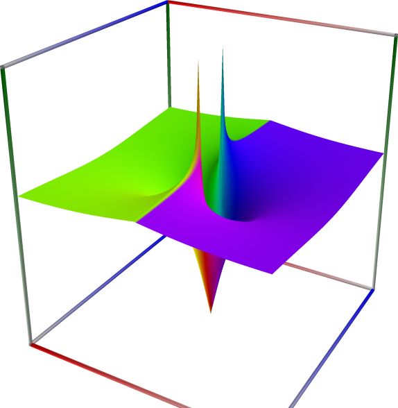
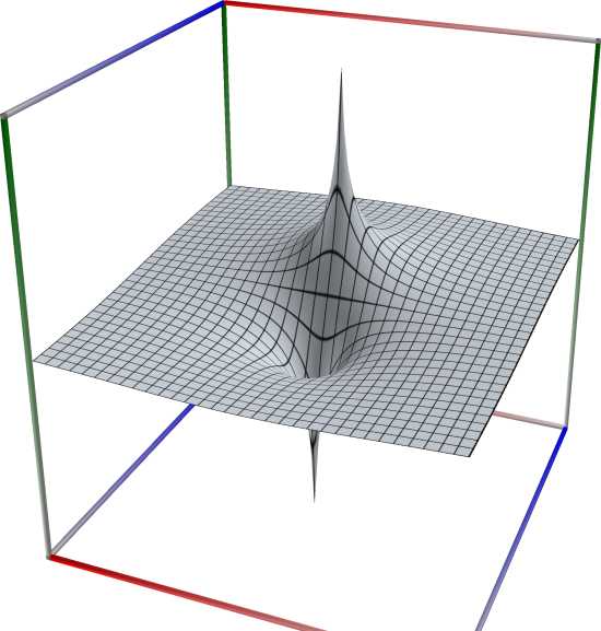
Left figure: real part of the Inverse Hyperbolic Tangent function. Camera angles are \(\theta=135^\circ\) and \(\phi = -12^\circ\), camera radius is -2.
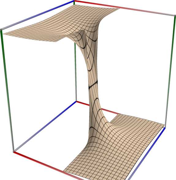
Middle figure: imaginary part of the Inverse Hyperbolic Tangent function. Camera angles are \(\theta=135^\circ\) and \(\phi = -12^\circ\), camera radius is -2.
Right figure: absolute value of the Inverse Hyperbolic Tangent function, with color-coded phase. Camera angles are \(\theta=135^\circ\) and \(\phi = -12^\circ\), camera radius is -2.
An example in Python
>>> from xlcalcnet import xreal
>>> xreal.Atanh(0.5)
xreal('5.2359877559829887307E-1')
>>> xreal.Atanh('0.51')
xreal('5.3518479027559984754E-1')
An example in Visual Basic
>>> from xlcalcnet import Gpr
>>> Gpr.Atanh(0.5)
Gpr('5.2359877559829887307E-1')
>>> Gpr.Atanh('0.51')
Gpr('5.3518479027559984754E-1')
An example with real input:
>>> from xlcalcnet import dec, mpm, ipm
>>> mpm.dps = 40; x = '0.5'
>>> \mathrm{d}x = dec.atanh(x); mx = mpm.atanh(x); ix = ipm.atanh(x)
>>> mpm.show([\mathrm{d}x, mx, ix])
dec:  5.493061443340548456976226184612628523237E-1
mpm:  5.493061443340548456976226184612628523237e-1
ipm:  5.493061443340548456976226184612628523237e-1 (2.09e-39%)

>>> from xlcalcnet import mpm, fpm, gmp, apm
>>> mpm.dps = 40; x = '0.5'
>>> fx = fpm.atanh(x); gx = gmp.atanh(x); ax = apm.atanh(x)
>>> mpm.show([fx, gx, ax])
fpm:  5.49306144334055E-01
gmp:  5.493061443340548456976226184612628523237E-01
apm:  5.493061443340548456976226184612628523237e-1 (2.09e-39%)
The following example with complex input shows that the relative error can be high in double precision:
>>> from xlcalcnet import dec, mpm, ipm
>>> mpm.dps = 20; z = '2 + 1.5E+2j'
>>> \mathrm{d}z = dec.atanh(z); mz = mpm.atanh(z); iz = ipm.atanh(z)
>>> mpm.show([\mathrm{d}z, mz, iz], aligned=True)
dec: 8.8869141126887266889E-5              + 1.5641309437602554673E+0j
mpm: 8.8869141126887266889e-5              + 1.5641309437602554673e+0j
ipm: 8.8869141126887268292e-5 (3.812e-15%) + 1.5641309437602554673e+0 (5.415e-20%)j

>>> from xlcalcnet import mpm, fpm, gmp, apm
>>> mpm.dps = 20; z = '2 + 1.5E+2j'
>>> fz = fpm.atanh(z); gz = gmp.atanh(z); az = apm.atanh(z)
>>> mpm.show([fz, gz, az], aligned=True)
fpm: 8.88691411268873E-05                 + 1.56413094376026E+00j
gmp: 8.8869141126887266889E-05            + 1.5641309437602554673E+00j
apm: 8.8869141126887266883e-5 (4.73e-17%) + 1.5641309437602554673e+0 (1.083e-19%)j
Inverse hyperbolic cotangent, \(\mathrm{acoth}(x)\)#
- ctx.acoth(x)#
Returns the inverse hyperbolic cotangent of \(x\), \(\mathrm{acoth}(x)\). See also Wikipedia [1367], MathWorld [960], NIST [511], Ehrhardt [309] (4.2.7), Mpmath [599].
The real inverse hyperbolic cotangent can be defined as \(\displaystyle \mathrm{acoth}(x) = \frac{1}{2} \log \left(\frac{x+1}{x-1} \right)\). The domain is the union of the open intervals \((-\infty, -1)\) and \((1, +\infty)\).
The complex inverse hyperbolic cotangent can be expressed in terms of related functions (with the principal-branch log and square root):
\[\mathrm{acoth}(z) = \frac{1}{2} \log \left(\frac{z+1}{z-1} \right) = \frac{1}{2} \left[ \log \left(1 + \frac{1}{z} \right) - \log \left(1 - \frac{1}{z} \right) \right]= \frac{1}{i} \mathrm{acot}(-iz).\]
 \(\quad\)
  \(\quad\)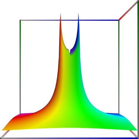
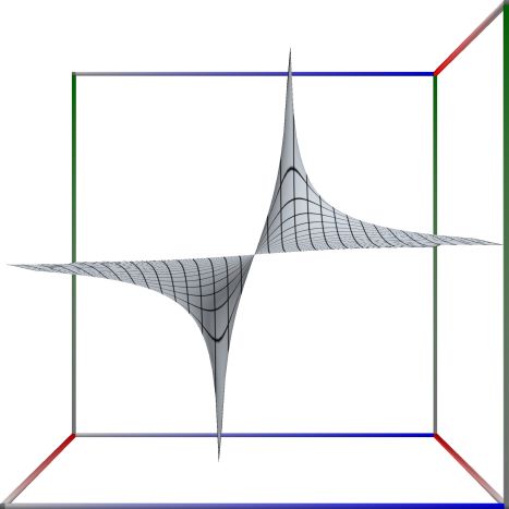
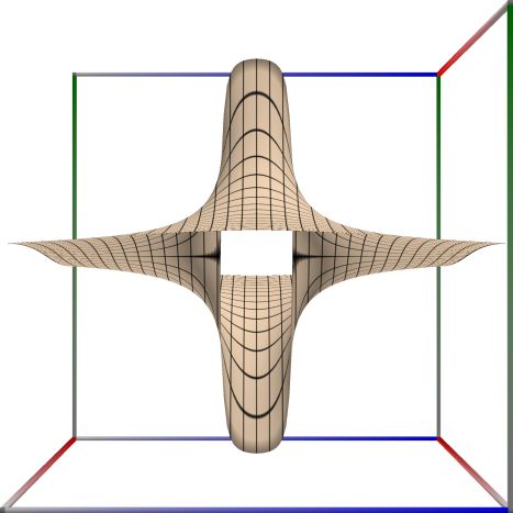
Left figure: real part of the Inverse Hyperbolic Cotangent function. Camera angles are \(\theta=135^\circ\) and \(\phi = -12^\circ\), camera radius is -2.
Middle figure: imaginary part of the Inverse Hyperbolic Cotangent function. Camera angles are \(\theta=135^\circ\) and \(\phi = -12^\circ\), camera radius is -2.
Right figure: absolute value of the Inverse Hyperbolic Cotangent function, with color-coded phase. Camera angles are \(\theta=135^\circ\) and \(\phi = -12^\circ\), camera radius is -2.
An example in Python
>>> from xlcalcnet import xreal
>>> xreal.Acoth(0.5)
xreal('5.2359877559829887307E-1')
>>> xreal.Acoth('0.51')
xreal('5.3518479027559984754E-1')
An example in Visual Basic
>>> from xlcalcnet import Gpr
>>> Gpr.Acoth(0.5)
Gpr('5.2359877559829887307E-1')
>>> Gpr.Acoth('0.51')
Gpr('5.3518479027559984754E-1')
An example with real input:
>>> from xlcalcnet import dec, mpm, ipm
>>> mpm.dps = 40; x = '1.5'
>>> \mathrm{d}x = dec.acoth(x); mx = mpm.acoth(x); ix = ipm.acoth(x)
>>> mpm.show([\mathrm{d}x, mx, ix])
dec:  8.047189562170501873003796666130938197628E-1
mpm:  8.047189562170501873003796666130938197628e-1
ipm:  8.047189562170501873003796666130938197628e-1 (2.853e-39%)

>>> from xlcalcnet import mpm, fpm, gmp, apm
>>> mpm.dps = 40; x = '1.5'
>>> fx = fpm.acoth(x); gx = gmp.acoth(x); ax = apm.acoth(x)
>>> mpm.show([fx, gx, ax])
fpm:  8.04718956217050E-01
gmp:  8.047189562170501873003796666130938197628E-01
apm:  8.047189562170501873003796666130938197628e-1 (7.133e-40%)
The following example with complex input shows that the relative error can be high in double precision:
>>> from xlcalcnet import dec, mpm, ipm
>>> mpm.dps = 20; z = '2 + 1.5E+2j'
>>> \mathrm{d}z = dec.acoth(z); mz = mpm.acoth(z); iz = ipm.acoth(z)
>>> mpm.show([\mathrm{d}z, mz, iz], aligned=True)
dec: 8.8869141126887266889E-5             - 6.6653830346411519558E-3j
mpm: 8.8869141126887266889e-5             - 6.6653830346411519558e-3j
ipm: 8.8869141126887267011e-5 (7.15e-16%) - 6.6653830346411519558e-3 (-1.489e-19%)j

>>> from xlcalcnet import mpm, fpm, gmp, apm
>>> mpm.dps = 20; z = '2 + 1.5E+2j'
>>> fz = fpm.acoth(z); gz = gmp.acoth(z); az = apm.acoth(z)
>>> mpm.show([fz, gz, az], aligned=True)
fpm: 8.88691411268873E-05                 - 6.66538303464115E-03j
gmp: 8.8869141126887266889E-05            - 6.6653830346411519558E-03j
apm: 8.8869141126887266888e-5 (1.28e-18%) - 6.6653830346411519558e-3 (-1.986e-19%)j
Inverse hyperbolic secant, \(\mathrm{asech}(x)\)#
- ctx.asech(x)#
where
ctxismath53,mathc53,ctxcpporctxflint.Returns the inverse hyperbolic secant of \(x\), \(\mathrm{asech}(x)\). See also Wikipedia [1367], MathWorld [961], NIST [511], Ehrhardt [309] (4.2.12), Mpmath [600].
The inverse hyperbolic secant can be defined as \(\displaystyle \mathrm{asech}(x) = \log \left(\frac{1}{x} + \sqrt{\frac{1}{x^2}-1} \right)\). The domain is the semi-open interval \((0, 1]\).
The inverse hyperbolic secant can be expressed in terms of related functions (with the principal-branch log and square root):
\[\mathrm{asech}(z) = \log \left(\frac{1}{z} + \sqrt{\frac{1}{z}+1} \sqrt{\frac{1}{z}-1}\right)\]
 \(\quad\)
  \(\quad\)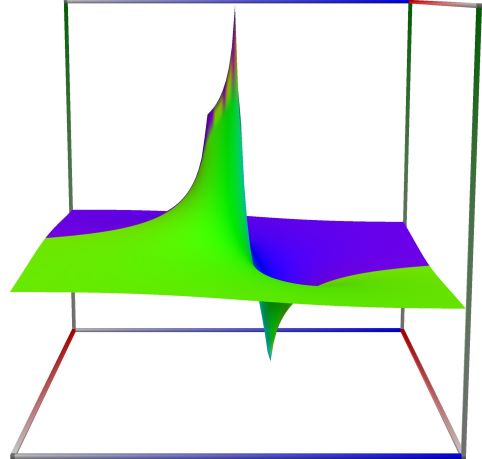
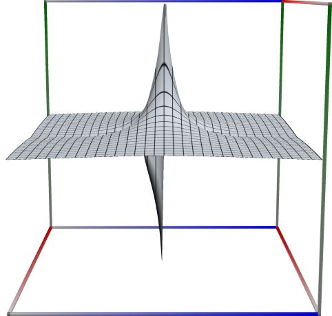
Left figure: real part of the Inverse Hyperbolic Secant function. Camera angles are \(\theta=135^\circ\) and \(\phi = -12^\circ\), camera radius is -2.
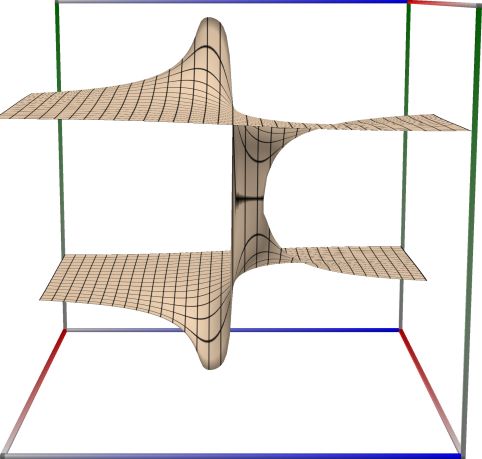
Middle figure: imaginary part of the Inverse Hyperbolic Secant function. Camera angles are \(\theta=135^\circ\) and \(\phi = -12^\circ\), camera radius is -2.
Right figure: absolute value of the Inverse Hyperbolic Secant function, with color-coded phase. Camera angles are \(\theta=135^\circ\) and \(\phi = -12^\circ\), camera radius is -2.
An example in Python
>>> from xlcalcnet import xreal
>>> xreal.Asech(0.5)
xreal('5.2359877559829887307E-1')
>>> xreal.Asech('0.51')
xreal('5.3518479027559984754E-1')
An example in Visual Basic
>>> from xlcalcnet import Gpr
>>> Gpr.Asech(0.5)
Gpr('5.2359877559829887307E-1')
>>> Gpr.Asech('0.51')
Gpr('5.3518479027559984754E-1')
An example with real input:
>>> from xlcalcnet import dec, mpm, ipm
>>> mpm.dps = 40; x = '0.5'
>>> \mathrm{d}x = dec.asech(x); mx = mpm.asech(x); ix = ipm.asech(x)
>>> mpm.show([\mathrm{d}x, mx, ix])
dec:  1.316957896924816708625046347307968444027E+0
mpm:  1.316957896924816708625046347307968444027e+0
ipm:  1.316957896924816708625046347307968444027e+0 (8.717e-40%)

>>> from xlcalcnet import mpm, fpm, gmp, apm
>>> mpm.dps = 40; x = '0.5'
>>> fx = fpm.asech(x); gx = gmp.asech(x); ax = apm.asech(x)
>>> mpm.show([fx, gx, ax])
fpm:  1.31695789692482E+00
gmp:  1.316957896924816708625046347307968444027E+00
apm:  1.316957896924816708625046347307968444027e+0 (8.717e-40%)
The following example with complex input shows that the relative error can be high in double precision:
>>> from xlcalcnet import dec, mpm, ipm
>>> mpm.dps = 20; z = '2 + 1.5E+2j'
>>> \mathrm{d}z = dec.asech(z); mz = mpm.asech(z); iz = ipm.asech(z)
>>> mpm.show([\mathrm{d}z, mz, iz], aligned=True)
dec: 6.6654323630640601125E-3              - 1.5707074556797408039E+0j
mpm: 6.6654323630640601125e-3              - 1.5707074556797408039e+0j
ipm: 6.6654323630640601131e-3 (5.053e-17%) - 1.5707074556797408039e+0 (-5.393e-20%)j

>>> from xlcalcnet import mpm, fpm, gmp, apm
>>> mpm.dps = 20; z = '2 + 1.5E+2j'
>>> fz = fpm.asech(z); gz = gmp.asech(z); az = apm.asech(z)
>>> mpm.show([fz, gz, az], aligned=True)
fpm: 6.66543236306406E-03                  - 1.57070745567974E+00j
gmp: 6.6654323630640601125E-03             - 1.5707074556797408039E+00j
apm: 6.6654323630640601124e-3 (1.787e-18%) - 1.5707074556797408039e+0 (-1.079e-19%)j
Inverse Hyperbolic Cosecant, \(\mathrm{acsch}(x)\)#
- ctx.acsch(x)#
where
ctxismath53,mathc53,ctxcpporctxflint.Returns the inverse hyperbolic cosecant of \(x\), \(\mathrm{acsch}(x)\). See also Wikipedia [1367], MathWorld [958], NIST [463], Ehrhardt [309] (4.2.10), Mpmath [597].
The real inverse hyperbolic cosecant can be defined as \(\displaystyle \mathrm{acsch}(x) = \log \left(\frac{1}{x} + \sqrt{\frac{1}{x^2}+1} \right)\). The domain is the real line with 0 removed.
The complex inverse hyperbolic cosecant can be expressed in terms of related functions (with the principal-branch log and square root):
\[\mathrm{acsch}(z) = \log \left(\frac{1}{z} + \sqrt{\frac{1}{z^2}+1} \right)\]
 \(\quad\)
  \(\quad\)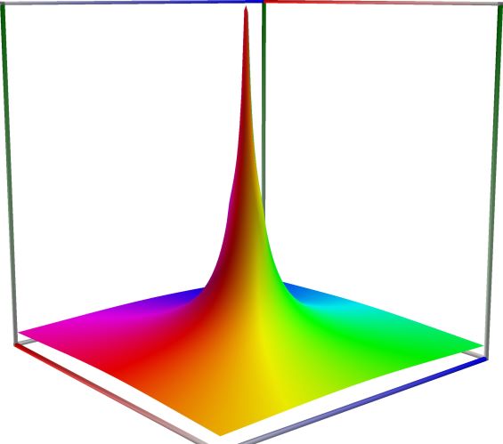
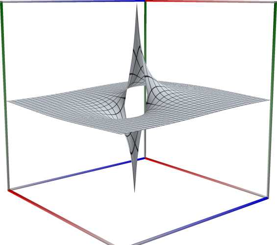
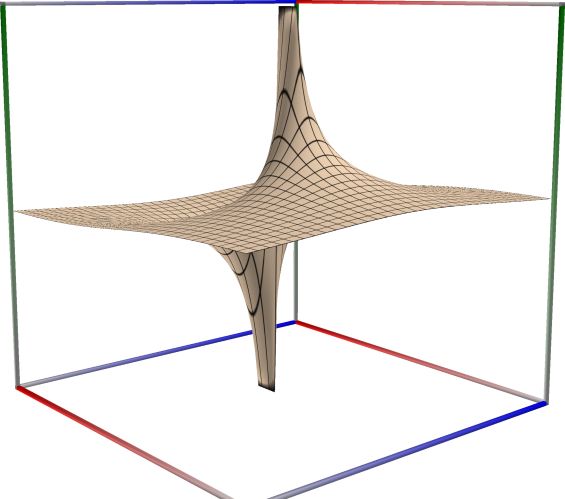
Left figure: real part of the Inverse Hyperbolic Cosecant function. Camera angles are \(\theta=135^\circ\) and \(\phi = -12^\circ\), camera radius is -2.
Middle figure: imaginary part of the Inverse Hyperbolic Cosecant function. Camera angles are \(\theta=135^\circ\) and \(\phi = -12^\circ\), camera radius is -2.
Right figure: absolute value of the Inverse Hyperbolic Cosecant function, with color-coded phase. Camera angles are \(\theta=135^\circ\) and \(\phi = -12^\circ\), camera radius is -2.
An example in Python
>>> from xlcalcnet import xreal
>>> xreal.Acsch(0.5)
xreal('5.2359877559829887307E-1')
>>> xreal.Acsch('0.51')
xreal('5.3518479027559984754E-1')
An example in Visual Basic
>>> from xlcalcnet import Gpr
>>> Gpr.Acsch(0.5)
Gpr('5.2359877559829887307E-1')
>>> Gpr.Acsch('0.51')
Gpr('5.3518479027559984754E-1')
An example with real input:
>>> from xlcalcnet import dec, mpm, ipm
>>> mpm.dps = 40; x = '1.5'
>>> \mathrm{d}x = dec.acsch(x); mx = mpm.acsch(x); ix = ipm.acsch(x)
>>> mpm.show([\mathrm{d}x, mx, ix])
dec:  6.251451172504166876342516732261024070342E-1
mpm:  6.251451172504166876342516732261024070342e-1
ipm:  6.251451172504166876342516732261024070342e-1 (1.01e-38%)

>>> from xlcalcnet import mpm, fpm, gmp, apm
>>> mpm.dps = 40; x = '1.5'
>>> fx = fpm.acsch(x); gx = gmp.acsch(x); ax = apm.acsch(x)
>>> mpm.show([fx, gx, ax])
fpm:  6.25145117250417E-01
gmp:  6.251451172504166876342516732261024070342E-01
apm:  6.251451172504166876342516732261024070342e-1 (9.181e-40%)
The following example with complex input shows that the relative error can be high in double precision:
>>> from xlcalcnet import dec, mpm, ipm
>>> mpm.dps = 20; z = '2 + 1.5E+2j'
>>> \mathrm{d}z = dec.acsch(z); mz = mpm.acsch(z); iz = ipm.acsch(z)
>>> mpm.show([\mathrm{d}z, mz, iz], aligned=True)
dec: 6.6654323630640601125E-3              - 1.5707074556797408039E+0j
mpm: 6.6654323630640601125e-3              - 1.5707074556797408039e+0j
ipm: 6.6654323630640601131e-3 (5.053e-17%) - 1.5707074556797408039e+0 (-5.393e-20%)j

>>> from xlcalcnet import mpm, fpm, gmp, apm
>>> mpm.dps = 20; z = '2 + 1.5E+2j'
>>> fz = fpm.acsch(z); gz = gmp.acsch(z); az = apm.acsch(z)
>>> mpm.show([fz, gz, az], aligned=True)
fpm: 6.66543236306406E-03                  - 1.57070745567974E+00j
gmp: 6.6654323630640601125E-03             - 1.5707074556797408039E+00j
apm: 6.6654323630640601124e-3 (1.787e-18%) - 1.5707074556797408039e+0 (-1.079e-19%)j