Hyperbolic functions

For a general introduction into hyperbolic functions, see Wikipedia [1344], NIST [510].

Hyperbolic sine, \(\mathrm{sinh}(x)\)

ctx.sinh(x)

where ctx is math53, mathc53, ctxcpp, ctxflint.

Returns the hyperbolic sine of \(x\), \(\sinh(x)\). See also Wikipedia [1344], MathWorld [938], NIST [510], Ehrhardt [309] (4.2.56), Flint [806], Flint [796], Mpmath [592].

The hyperbolic sine can be expressed in terms of the exponential function as \(\displaystyle \sinh(x) = \frac{e^x - e^{-x}}{2} = \frac{e^{2x-1}}{2e^x} = \frac{1-e^{-2x}}{2e^x}\).

The complex hyperbolic sine can be expressed in terms of related functions:

\[\sinh(z) = \frac{e^z - e^{-z}}{2} = \frac{e^{2z-1}}{2e^z} = \frac{1-e^{-2z}}{2e^z} = -i \sin(iz)\]

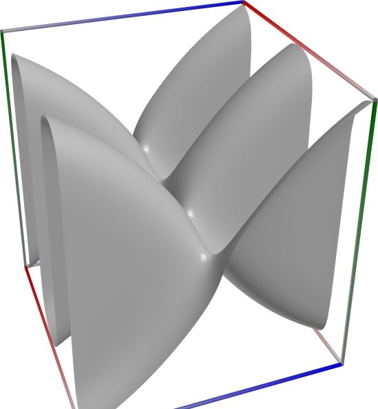\(\quad\) 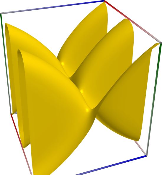\(\quad\)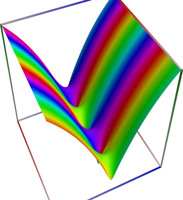

Left figure: real part of the Hyperbolic Sine function. Camera angles are \(\theta=135^\circ\) and \(\phi = -12^\circ\), camera radius is -2.

Middle figure: imaginary part of the Hyperbolic Sine function. Camera angles are \(\theta=135^\circ\) and \(\phi = -12^\circ\), camera radius is -2.

Right figure: absolute value of the Hyperbolic Sine function, with color-coded phase. Camera angles are \(\theta=135^\circ\) and \(\phi = -12^\circ\), camera radius is -2.

An example in Python

>>> from xlcalcnet import xreal
>>> xreal.Sinh(0.5)
xreal('5.2359877559829887307E-1')
>>> xreal.Sinh('0.51')
xreal('5.3518479027559984754E-1')

An example in Visual Basic

>>> from xlcalcnet import Gpr
>>> Gpr.Sinh(0.5)
Gpr('5.2359877559829887307E-1')
>>> Gpr.Sinh('0.51')
Gpr('5.3518479027559984754E-1')

An example with real input:

>>> from xlcalcnet import dec, mpm, ipm
>>> mpm.dps = 40; x = '3.14159265358979'
>>> \mathrm{d}x = dec.sinh(x); mx = mpm.sinh(x); ix = ipm.sinh(x)
>>> mpm.show([\mathrm{d}x, mx, ix])
dec:  1.154873935725771083786968769455998476991E+1
mpm:  1.154873935725771083786968769455998476991e+1
ipm:  1.154873935725771083786968769455998476991e+1 (3.181e-39%)

>>> from xlcalcnet import mpm, fpm, gmp, apm
>>> mpm.dps = 40; x = '3.14159265358979'
>>> fx = fpm.sinh(x); gx = gmp.sinh(x); ax = apm.sinh(x)
>>> mpm.show([fx, gx, ax])
fpm:  1.15487393572577E+01
gmp:  1.154873935725771083786968769455998476991E+01
apm:  1.154873935725771083786968769455998476991e+1 (3.181e-39%)

The following example with complex input shows that the relative error can be high in double precision:

>>> from xlcalcnet import dec, mpm, ipm
>>> mpm.dps = 20; z = '1.5E+2 - 1.57079632679489j'
>>> \mathrm{d}z = dec.sinh(z); mz = mpm.sinh(z); iz = ipm.sinh(z)
>>> mpm.show([\mathrm{d}z, mz, iz], aligned=True)
dec: 4.6126430548443107461E+50            - 6.9685479033318984866E+64j
mpm: 4.6126426732366959851e+50            - 6.9685479033318984866e+64j
ipm: 4.6126432634956628493e+50 (1.28e-5%) - 6.9685479033318984866e+64 (-6.4e-20%)j

>>> from xlcalcnet import mpm, fpm, gmp, apm
>>> mpm.dps = 20; z = '1.5E+2 - 1.57079632679489j'
>>> fz = fpm.sinh(z); gz = gmp.sinh(z); az = apm.sinh(z)
>>> mpm.show([fz, gz, az], aligned=True)
fpm: 4.68465544771206E+50                 - 6.96854790333190E+64j
gmp: 4.6126426732366959851E+50            - 6.9685479033318984866E+64j
apm: 4.6126430605941429898e+50 (1.32e-5%) - 6.9685479033318984866e+64 (-6.4e-20%)j

From mpmath:

>>> from xlcalcnet import dec, mpr, ivr, ivc
>>> ivr.dps = 25; ivr.pretty = True
>>> sinh(2+3j)
(-3.590564589985779952012565 + 0.5309210862485198052670401j)
>>> j*sin(3-2j)
(-3.590564589985779952012565 + 0.5309210862485198052670401j)

Hyperbolic cosine, \(\mathrm{cosh}(x)\)

ctx.cosh(x)

where ctx is math53, mathc53, ctxcpp, ctxflint.

Returns the hyperbolic cosine of \(x\), \(\cosh(x)\). See also Wikipedia [1344], MathWorld [935], NIST [510], Ehrhardt [309] (4.2.20), Flint [806], Flint [796], Mpmath [589].

The hyperbolic cosine can be expressed in terms of the exponential function as \(\displaystyle \cosh(x) = \frac{e^x + e^{-x}}{2} = \frac{e^{2x+1}}{2e^x} = \frac{1+e^{-2x}}{2e^x}\).

The complex hyperbolic cosine can be expressed in terms of related functions:

\[\cosh(z) = \frac{e^z + e^{-z}}{2} = \frac{e^{2z+1}}{2e^z} = \frac{1+e^{-2z}}{2e^z} = \cos(iz)\]

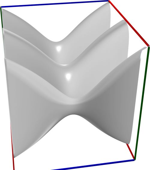\(\quad\) \(\quad\)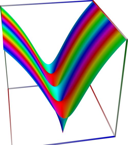

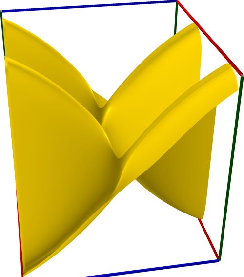
Left figure: real part of the Hyperbolic Cosine function. Camera angles are \(\theta=135^\circ\) and \(\phi = -12^\circ\), camera radius is -2.

Middle figure: imaginary part of the Hyperbolic Cosine function. Camera angles are \(\theta=135^\circ\) and \(\phi = -12^\circ\), camera radius is -2.

Right figure: absolute value of the Hyperbolic Cosine function, with color-coded phase. Camera angles are \(\theta=135^\circ\) and \(\phi = -12^\circ\), camera radius is -2.

An example in Python

>>> from xlcalcnet import xreal
>>> xreal.Cosh(0.5)
xreal('5.2359877559829887307E-1')
>>> xreal.Cosh('0.51')
xreal('5.3518479027559984754E-1')

An example in Visual Basic

>>> from xlcalcnet import Gpr
>>> Gpr.Cosh(0.5)
Gpr('5.2359877559829887307E-1')
>>> Gpr.Cosh('0.51')
Gpr('5.3518479027559984754E-1')

An example with real input:

>>> from xlcalcnet import dec, mpm, ipm
>>> mpm.dps = 40; x = '1.57079632679489'
>>> \mathrm{d}x = dec.cosh(x); mx = mpm.cosh(x); ix = ipm.cosh(x)
>>> mpm.show([\mathrm{d}x, mx, ix])
dec:  6.619231321691639751442098584651351473054E-15
mpm:  6.619231321691639751442098575708073666164e-15
ipm:  6.619231321691639751442098587187510685913e-15 (1.734e-25%)

>>> from xlcalcnet import mpm, fpm, gmp, apm
>>> mpm.dps = 40; x = '1.57079632679489'
>>> fx = fpm.cosh(x); gx = gmp.cosh(x); ax = apm.cosh(x)
>>> mpm.show([fx, gx, ax])
fpm:  6.72257048770831E-15
gmp:  6.619231321691639751442098575708073666164E-15
apm:  6.619231321691639751442098584676383837843e-15 (1.768e-25%)

The following example with complex input shows that the relative error can be high in double precision:

>>> from xlcalcnet import dec, mpm, ipm
>>> mpm.dps = 20; z = '1.5E+2 - 3.14159265358979j'
>>> \mathrm{d}z = dec.cosh(z); mz = mpm.cosh(z); iz = ipm.cosh(z)
>>> mpm.show([\mathrm{d}z, mz, iz], aligned=True)
dec: -6.9685479033318984866E+64             - 2.2567382063567230055E+50j
mpm: -6.9685479033318984866e+64             - 2.2567375654278714043e+50j
ipm: -6.9685479033318984866e+64 (-6.4e-20%) - 2.2567387459458051327e+50 (-5.231e-5%)j

>>> from xlcalcnet import mpm, fpm, gmp, apm
>>> mpm.dps = 20; z = '1.5E+2 - 3.14159265358979j'
>>> fz = fpm.cosh(z); gz = gmp.cosh(z); az = apm.cosh(z)
>>> mpm.show([fz, gz, az], aligned=True)
fpm: -6.96854790333190E+64                  - 2.25159995138029E+50j
gmp: -6.9685479033318984866E+64             - 2.2567375654278714043E+50j
apm: -6.9685479033318984866e+64 (-6.4e-20%) - 2.2567382294692091265e+50 (-5.406e-5%)j

Generalized to complex numbers, the hyperbolic cosine is equivalent to a cosine with the argument rotated in the imaginary direction, or \(\cosh x = \cos ix\):

>>> from xlcalcnet import dec, mpr, ivr, ivc
>>> ivr.dps = 25; ivr.pretty = True
>>> cosh(2+3j)
(-3.724545504915322565473971 + 0.5118225699873846088344638j)
>>> cos(3-2j)
(-3.724545504915322565473971 + 0.5118225699873846088344638j)

Hyperbolic tangent, \(\mathrm{tanh}(x)\)

ctx.tanh(x)

where ctx is math53, mathc53, ctxcpp or ctxflint.

Returns the hyperbolic tangent of \(x\), \(\tanh(x)\). See also Wikipedia [1344], MathWorld [939], NIST [510], Ehrhardt [309] (4.2.62), Flint [806], Flint [796], Mpmath [593].

The hyperbolic tangent can be expressed in terms of the exponential function as \(\displaystyle \tanh(x) = \frac{\sinh(x)}{\cosh(x)}= \frac{e^x - e^{-x}}{e^x + e^{-x}} = \frac{e^{2x-1}}{e^{2x+1}}\).

The complex hyperbolic tangent can be expressed in terms of related functions:

\[\tanh(z) = \frac{\sinh(z)}{\cosh(z)}= \frac{e^z - e^{-z}}{e^z + e^{-z}} = \frac{e^{2z-1}}{e^{2z+1}} = -i \tan(iz)\]

\(\quad\) \(\quad\)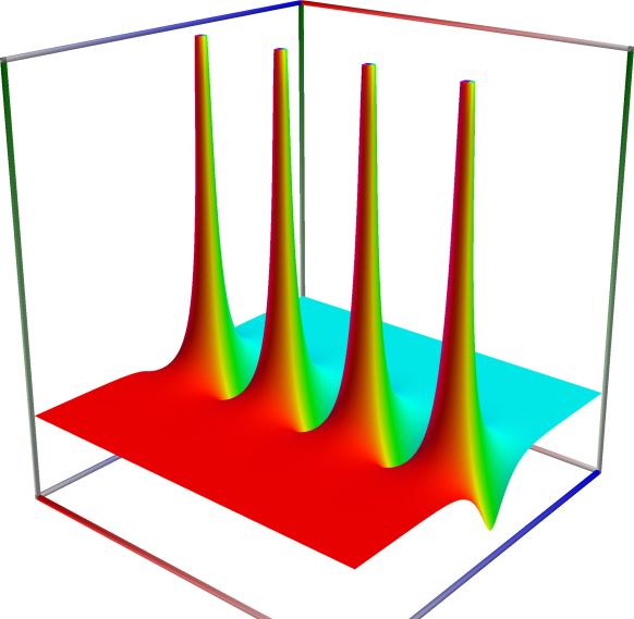

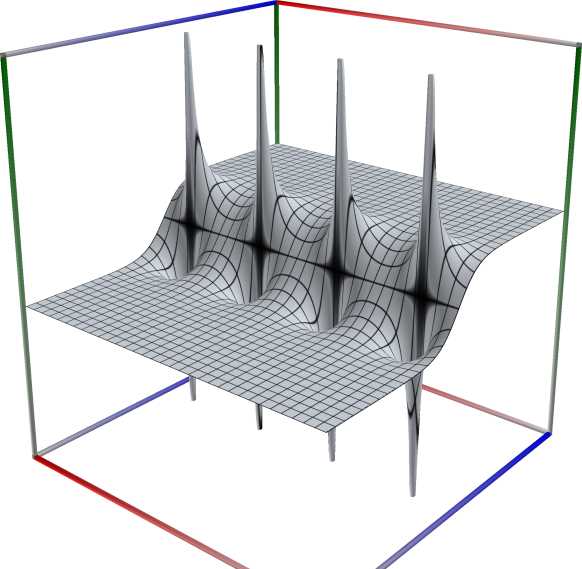
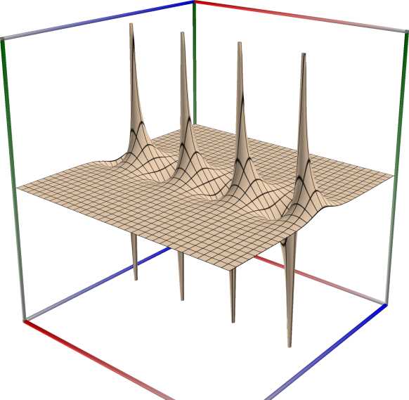
Left figure: real part of the Hyperbolic Tangent function. Camera angles are \(\theta=135^\circ\) and \(\phi = -12^\circ\), camera radius is -2.

Middle figure: imaginary part of the Hyperbolic Tangent function. Camera angles are \(\theta=135^\circ\) and \(\phi = -12^\circ\), camera radius is -2.

Right figure: absolute value of the Hyperbolic Tangent function, with color-coded phase. Camera angles are \(\theta=135^\circ\) and \(\phi = -12^\circ\), camera radius is -2.

An example in Python

>>> from xlcalcnet import xreal
>>> xreal.Tanh(0.5)
xreal('5.2359877559829887307E-1')
>>> xreal.Tanh('0.51')
xreal('5.3518479027559984754E-1')

An example in Visual Basic

>>> from xlcalcnet import Gpr
>>> Gpr.Tanh(0.5)
Gpr('5.2359877559829887307E-1')
>>> Gpr.Tanh('0.51')
Gpr('5.3518479027559984754E-1')

An example with real input:

>>> from xlcalcnet import dec, mpm, ipm
>>> mpm.dps = 40; x = '1.57079632679489'
>>> \mathrm{d}x = dec.tanh(x); mx = mpm.tanh(x); ix = ipm.tanh(x)
>>> mpm.show([\mathrm{d}x, mx, ix])
dec:  9.171523356672732950300364697768401207429E-1
mpm:  9.171523356672732950300364697768401207429e-1
ipm:  9.171523356672732950300364697768401207429e-1 (8.136e-39%)

>>> from xlcalcnet import mpm, fpm, gmp, apm
>>> mpm.dps = 40; x = '1.57079632679489'
>>> fx = fpm.tanh(x); gx = gmp.tanh(x); ax = apm.tanh(x)
>>> mpm.show([fx, gx, ax])
fpm:  9.17152335667273E-01
gmp:  9.171523356672732950300364697768401207429E-01
apm:  9.171523356672732950300364697768401207429e-1 (1.252e-39%)

The following example with complex input shows that the relative error can be high in double precision:

>>> from xlcalcnet import dec, mpm, ipm
>>> mpm.dps = 20; z = '0.001 - 1.57079632679489j'
>>> \mathrm{d}z = dec.tanh(z); mz = mpm.tanh(z); iz = ipm.tanh(z)
>>> mpm.show([\mathrm{d}z, mz, iz], aligned=True)
dec: 1.0000003333333111111E+3              - 6.6192291152816404696E-9j
mpm: 1.0000003333333111111e+3              - 6.6192285676675710077e-9j
ipm: 1.0000003333333111111e+3 (6.505e-19%) - 6.6192294147002359176e-9 (-1.28e-5%)j

>>> from xlcalcnet import mpm, fpm, gmp, apm
>>> mpm.dps = 20; z = '0.001 - 1.57079632679489j'
>>> fz = fpm.tanh(z); gz = gmp.tanh(z); az = apm.tanh(z)
>>> mpm.show([fz, gz, az], aligned=True)
fpm: 1.00000033333331E+03                  - 6.72256824685193E-09j
gmp: 1.0000003333333111111E+03             - 6.6192285676675710076E-09j
apm: 1.0000003333333111111e+3 (1.301e-19%) - 6.6192291235327573548e-9 (-1.32e-5%)j

Hyperbolic cotangent, \(\mathrm{coth}(x)\)

ctx.coth(x)

where ctx is math53, mathc53, ctxcpp or ctxflint.

Returns the hyperbolic cotangent of \(x\), \(\mathrm{coth}(x)\). See also Wikipedia [1344], MathWorld [936], NIST [510], Ehrhardt [309] (4.2.22), Flint [806], Flint [796], Mpmath [590].

The hyperbolic cotangent can be expressed in terms of related functions as \(\displaystyle \mathrm{coth}(x) = \frac{\cosh(x)}{ \sinh(x)}= \frac{e^x + e^{-x}}{e^x - e^{-x}} = \frac{e^{2x+1}}{e^{2x-1}}\).

The complex hyperbolic cotangent can be expressed in terms of related functions:

\[\mathrm{coth}(z) = \frac{\cosh(z)}{ \sinh(z)}= \frac{e^z + e^{-z}}{e^z - e^{-z}} = \frac{e^{2z+1}}{e^{2z-1}} = i \cdot \cot(iz)\]

\(\quad\) \(\quad\)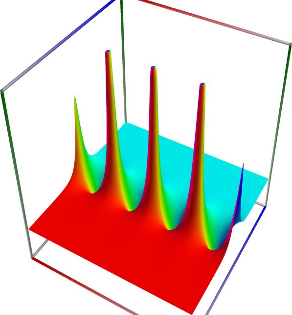

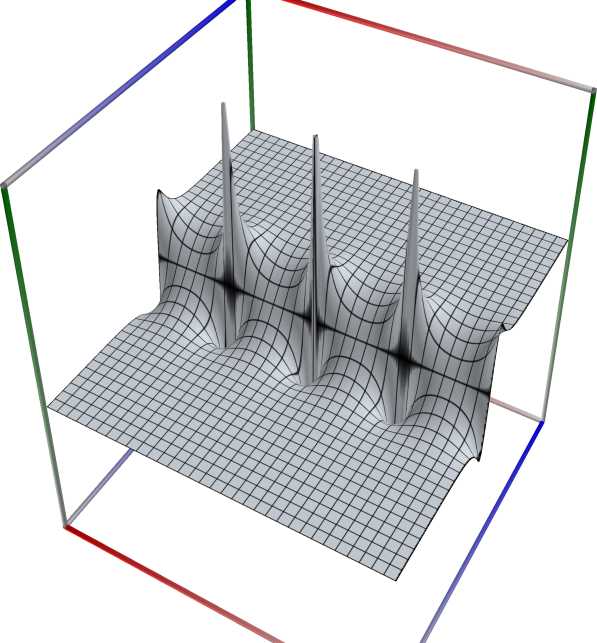
Left figure: real part of the Hyperbolic Cotangent function. Camera angles are \(\theta=135^\circ\) and \(\phi = -12^\circ\), camera radius is -2.

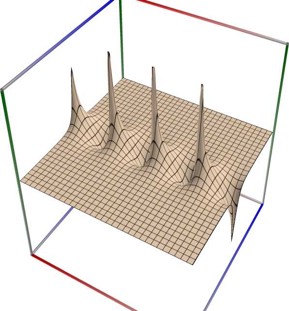
Middle figure: imaginary part of the Hyperbolic Cotangent function. Camera angles are \(\theta=135^\circ\) and \(\phi = -12^\circ\), camera radius is -2.

Right figure: absolute value of the Hyperbolic Cotangent function, with color-coded phase. Camera angles are \(\theta=135^\circ\) and \(\phi = -12^\circ\), camera radius is -2.

An example in Python

>>> from xlcalcnet import xreal
>>> xreal.Coth(0.5)
xreal('5.2359877559829887307E-1')
>>> xreal.Coth('0.51')
xreal('5.3518479027559984754E-1')

An example in Visual Basic

>>> from xlcalcnet import Gpr
>>> Gpr.Coth(0.5)
Gpr('5.2359877559829887307E-1')
>>> Gpr.Coth('0.51')
Gpr('5.3518479027559984754E-1')

An example with real input:

>>> from xlcalcnet import dec, mpm, ipm
>>> mpm.dps = 40; x = '1.57079632679489'
>>> \mathrm{d}x = dec.coth(x); mx = mpm.coth(x); ix = ipm.coth(x)
>>> mpm.show([\mathrm{d}x, mx, ix])
dec:  1.090331410727369479890382783582027249153E+0
mpm:  1.090331410727369479890382783582027249153e+0
ipm:  1.090331410727369479890382783582027249153e+0 (9.476e-39%)

>>> from xlcalcnet import mpm, fpm, gmp, apm
>>> mpm.dps = 40; x = '1.57079632679489'
>>> fx = fpm.coth(x); gx = gmp.coth(x); ax = apm.coth(x)
>>> mpm.show([fx, gx, ax])
fpm:  1.09033141072737E+00
gmp:  1.090331410727369479890382783582027249153E+00
apm:  1.090331410727369479890382783582027249153e+0 (1.053e-39%)

The following example with complex input shows that the relative error can be high in double precision:

>>> from xlcalcnet import dec, mpm, ipm
>>> mpm.dps = 20; z = '0.001 - 1.57079632679489j'
>>> \mathrm{d}z = dec.coth(z); mz = mpm.coth(z); iz = ipm.coth(z)
>>> mpm.show([\mathrm{d}z, mz, iz], aligned=True)
dec: 9.9999966666679999995E-4              + 6.6192247024647308782E-15j
mpm: 9.9999966666679999995e-4              + 6.6192241548510264921e-15j
ipm: 9.9999966666679999995e-4 (4.963e-19%) + 6.6192250018831267140e-15 (1.28e-5%)j

>>> from xlcalcnet import mpm, fpm, gmp, apm
>>> mpm.dps = 20; z = '0.001 - 1.57079632679489j'
>>> fz = fpm.coth(z); gz = gmp.coth(z); az = apm.coth(z)
>>> mpm.show([fz, gz, az], aligned=True)
fpm: 9.99999666666800E-04                  + 6.72256376514230E-15j
gmp: 9.9999966666679999995E-04             + 6.6192241548510264921E-15j
apm: 9.9999966666679999995e-4 (1.654e-19%) + 6.6192247107158422627e-15 (1.32e-5%)j

Hyperbolic cosecant, \(\mathrm{csch}(x)\)

ctx.csch(x)

where ctx is math53, mathc53, ctxcpp or ctxflint.

Returns the hyperbolic cosecant of \(x\), \(\mathrm{csch}(x)\). See also Wikipedia [1344], MathWorld [934], NIST [510], Ehrhardt [309] (4.2.24), Flint [806], Flint [796], Mpmath [588].

The hyperbolic cosecant can be expressed in terms of the exponential function as \(\displaystyle \mathrm{csch}(x) = \frac{1}{\sinh(x)}= \frac{2}{e^x - e^{-x}} = \frac{2e^x}{1 - e^{-2x}}\).

The complex hyperbolic cosecant can be expressed in terms of related functions:

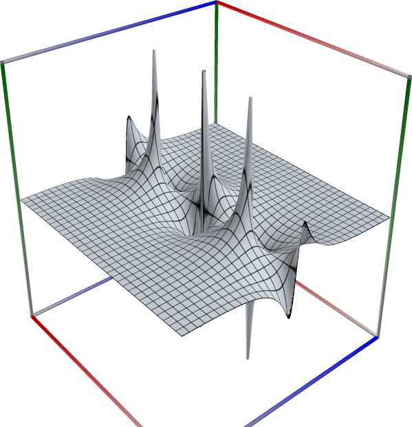
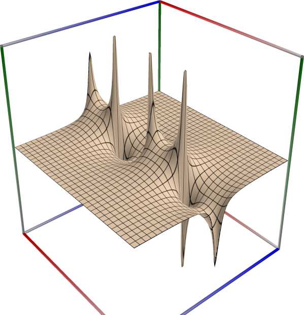
\[\mathrm{csch}(z) = \frac{1}{\sinh(z)}= \frac{2}{e^z - e^{-z}} = \frac{2e^z}{1 - e^{-2z}} = i \cdot \mathrm{csc}(iz)\]

\(\quad\) \(\quad\)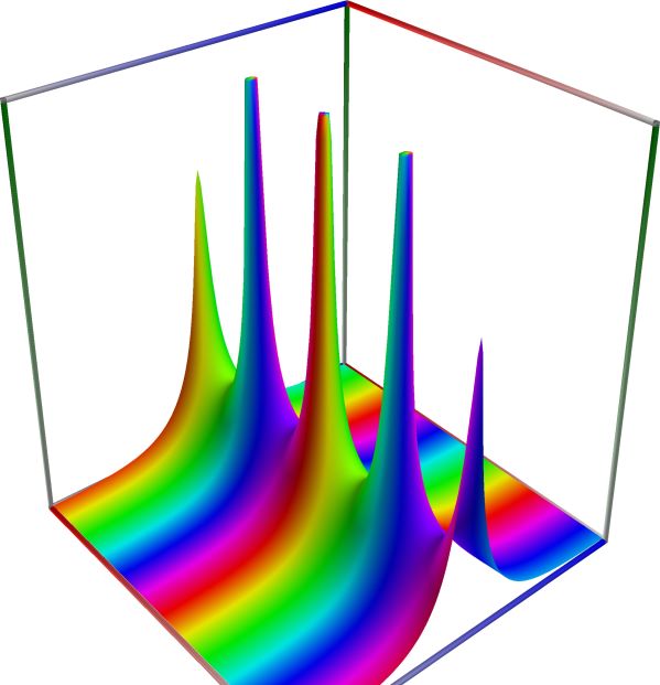

Left figure: real part of the Hyperbolic Cosecant function. Camera angles are \(\theta=135^\circ\) and \(\phi = -12^\circ\), camera radius is -2.

Middle figure: imaginary part of the Hyperbolic Cosecant function. Camera angles are \(\theta=135^\circ\) and \(\phi = -12^\circ\), camera radius is -2.

Right figure: absolute value of the Hyperbolic Cosecant function, with color-coded phase. Camera angles are \(\theta=135^\circ\) and \(\phi = -12^\circ\), camera radius is -2.

An example in Python

>>> from xlcalcnet import xreal
>>> xreal.Csch(0.5)
xreal('5.2359877559829887307E-1')
>>> xreal.Csch('0.51')
xreal('5.3518479027559984754E-1')

An example in Visual Basic

>>> from xlcalcnet import Gpr
>>> Gpr.Csch(0.5)
Gpr('5.2359877559829887307E-1')
>>> Gpr.Csch('0.51')
Gpr('5.3518479027559984754E-1')

An example with real input:

>>> from xlcalcnet import dec, mpm, ipm
>>> mpm.dps = 40; x = '3.14159265358979'
>>> \mathrm{d}x = dec.csch(x); mx = mpm.csch(x); ix = ipm.csch(x)
>>> mpm.show([\mathrm{d}x, mx, ix])
dec:  8.658953753004722329472715990465035467380E-2
mpm:  8.658953753004722329472715990465035467381e-2
ipm:  8.658953753004722329472715990465035467380e-2 (7.457e-39%)

>>> from xlcalcnet import mpm, fpm, gmp, apm
>>> mpm.dps = 40; x = '3.14159265358979'
>>> fx = fpm.csch(x); gx = gmp.csch(x); ax = apm.csch(x)
>>> mpm.show([fx, gx, ax])
fpm:  8.65895375300472E-02
gmp:  8.658953753004722329472715990465035467381E-02
apm:  8.658953753004722329472715990465035467380e-2 (3.314e-39%)

The following example with complex input shows that the relative error can be high in double precision:

>>> from xlcalcnet import dec, mpm, ipm
>>> mpm.dps = 20; z = '1.5E+2 - 1.57079632679489j'
>>> \mathrm{d}z = dec.csch(z); mz = mpm.csch(z); iz = ipm.csch(z)
>>> mpm.show([\mathrm{d}z, mz, iz], aligned=True)
dec: 9.4987240003426845058E-80            + 1.4350191946328820840E-65j
mpm: 9.4987232145057216312e-80            + 1.4350191946328820840e-65j
ipm: 9.4987244300142594276e-80 (1.28e-5%) + 1.4350191946328820840e-65 (5.605e-20%)j

>>> from xlcalcnet import mpm, fpm, gmp, apm
>>> mpm.dps = 20; z = '1.5E+2 - 1.57079632679489j'
>>> fz = fpm.csch(z); gz = gmp.csch(z); az = apm.csch(z)
>>> mpm.show([fz, gz, az], aligned=True)
fpm: 9.64701768713396E-80                  + 1.43501919463288E-65j
gmp: 9.4987232145057216313E-80             + 1.4350191946328820840E-65j
apm: 9.4987240121831995601e-80 (1.326e-5%) + 1.4350191946328820840e-65 (5.605e-20%)j

Hyperbolic secant, \(\mathrm{sech}(x)\)

ctx.sech(x)

where ctx is math53, mathc53, ctxcpp or ctxflint.

Returns the hyperbolic secant of \(x\), \(\mathrm{sech}(x)\). See also Wikipedia [1344], MathWorld [937], NIST [510], Ehrhardt [309] (4.2.54), Mpmath [591].

The hyperbolic secant can be expressed in terms of the exponential function as \(\displaystyle \mathrm{sech}(x) = \frac{1}{ \cosh(x)}= \frac{2}{e^x + e^{-x}} = \frac{2e^x}{e^{2x}+1}\).

The complex hyperbolic secant can be expressed in terms of related functions:

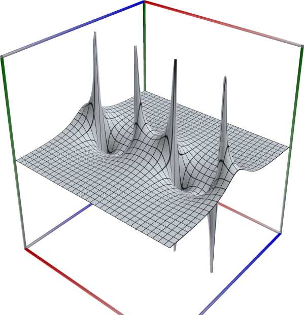
\[\mathrm{sech}(z) = \frac{1}{ \cosh(z)}= \frac{2}{e^z + e^{-z}} = \frac{2e^z}{e^{2z}+1} = \mathrm{sec}(iz)\]

\(\quad\) \(\quad\)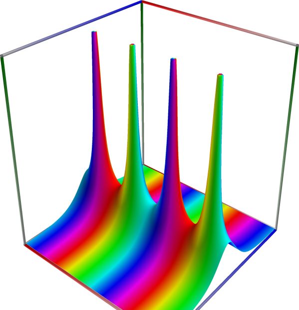

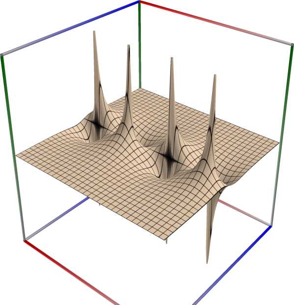
Left figure: real part of the Hyperbolic Secant function. Camera angles are \(\theta=135^\circ\) and \(\phi = -12^\circ\), camera radius is -2.

Middle figure: imaginary part of the Hyperbolic Secant function. Camera angles are \(\theta=135^\circ\) and \(\phi = -12^\circ\), camera radius is -2.

Right figure: absolute value of the Hyperbolic Secant function, with color-coded phase. Camera angles are \(\theta=135^\circ\) and \(\phi = -12^\circ\), camera radius is -2.

An example in Python

>>> from xlcalcnet import xreal
>>> xreal.Sech(0.5)
xreal('5.2359877559829887307E-1')
>>> xreal.Sech('0.51')
xreal('5.3518479027559984754E-1')

An example in Visual Basic

>>> from xlcalcnet import Gpr
>>> Gpr.Sech(0.5)
Gpr('5.2359877559829887307E-1')
>>> Gpr.Sech('0.51')
Gpr('5.3518479027559984754E-1')

An example with real input:

>>> from xlcalcnet import dec, mpm, ipm
>>> mpm.dps = 40; x = '1.57079632679489'
>>> \mathrm{d}x = dec.sech(x); mx = mpm.sech(x); ix = ipm.sech(x)
>>> mpm.show([\mathrm{d}x, mx, ix])
dec:  3.985368153383890998882443018904163666217E-1
mpm:  3.985368153383890998882443018904163666217e-1
ipm:  3.985368153383890998882443018904163666217e-1 (4.321e-39%)

>>> from xlcalcnet import mpm, fpm, gmp, apm
>>> mpm.dps = 40; x = '1.57079632679489'
>>> fx = fpm.sech(x); gx = gmp.sech(x); ax = apm.sech(x)
>>> mpm.show([fx, gx, ax])
fpm:  3.98536815338389E-01
gmp:  3.985368153383890998882443018904163666217E-01
apm:  3.985368153383890998882443018904163666217e-1 (2.16e-39%)

The following example with complex input shows that the relative error can be high in double precision:

>>> from xlcalcnet import dec, mpm, ipm
>>> mpm.dps = 20; z = '1.5E+2 - 3.14159265358979j'
>>> \mathrm{d}z = dec.sech(z); mz = mpm.sech(z); iz = ipm.sech(z)
>>> mpm.show([\mathrm{d}z, mz, iz], aligned=True)
dec: -1.4350191946328820840E-65               + 4.6472560543565481719E-80j
mpm: -1.4350191946328820840e-65               + 4.6472547345045256263e-80j
ipm: -1.4350191946328820840e-65 (-5.605e-20%) + 4.6472571655216012191e-80 (5.231e-5%)j

>>> from xlcalcnet import mpm, fpm, gmp, apm
>>> mpm.dps = 20; z = '1.5E+2 - 3.14159265358979j'
>>> fz = fpm.sech(z); gz = gmp.sech(z); az = apm.sech(z)
>>> mpm.show([fz, gz, az], aligned=True)
fpm: -1.43501919463288E-65                    + 4.63667494819155E-80j
gmp: -1.4350191946328820840E-65               + 4.6472547345045256263E-80j
apm: -1.4350191946328820840e-65 (-5.605e-20%) + 4.6472561019516306473e-80 (5.401e-5%)j