Ctrl+K

XlCalcNet Documentation

  • Preface

Getting started

  • Setup and general usage
    • Setting up XlCalcNet
    • General and user interface functions
    • Calling Python from C#
    • Using XlCalcNet with spreadsheet formulas
    • Mathematical functions based on Mpmath, Gmpy2 and Python-Flint (only Python)
    • Mathematical functions in fixed precision
    • Mathematical functions based on XlCalcNet2
    • A quick look at Numpy
    • A quick look at Matplotlib and related libraries
    • A quick look at Pandas and Xlxswriter
    • A quick look at Scipy
    • A quick look at R, RStudio and Rpy2
  • Basic floating point functions
    • Operator overloading, general real functions
    • Machine constants, general
    • Properties of numbers
    • Integer related functions
    • Floating point functions for real numbers
    • Fraction and remainder related functions
    • Functions related to mantissa width and exponent range
    • Mathematical Constants
  • Elementary scalar functions (real and complex)
    • Complex components
    • Roots and quadratic, cubic, and quartic equations
    • Exponential and related functions
    • Logarithms and related functions
    • Power functions
    • Trigonometric functions, in radians
    • Trigonometric functions, in multiples of \(\pi\)
    • Hyperbolic functions
    • Inverse trigonometric functions, in radians
    • Inverse hyperbolic functions
    • Factorials, Gamma and related functions
    • Miscellaneous functions
  • Statistical Distributions
    • Introduction to random variables and distributions
    • Base class for univariate distributions
    • Base class for continuous univariate distributions
    • Base class for discrete univariate distributions
    • Closed form distributions, based on elementary functions
      • Boost: Arcsine Distribution
      • Boost: Cauchy distribution
      • Boost: Exponential distribution
      • Boost: Gumbel (Generalized Extreme Value distribution Type-I) distribution
      • Boost: Hyperexponential Distribution
      • !!!Boost: Kumaraswamy distribution
      • Boost: Laplace distribution
      • Boost: Logistic distribution
      • Boost: Pareto distribution
      • Boost: Rayleigh distribution
      • Boost: Triangular Distribution
      • Boost: Uniform distribution
      • Boost: Weibull (Minimum-Type-III) distribution
      • Dagum (Burr Type III) distribution
      • Fisk (log-logistic) distribution
      • Fréchet (Maximum/Minimum-Type-II or Inverse Weibull) distribution
      • Generalized Extreme Value (Maximum) or GEV distribution
      • Generalized Pareto distribution
      • Gompertz-Makeham distribution
      • Lomax distribution
      • Shifted Gompertz distribution
      • Singh-Maddala (Burr Type XII) distribution
    • Closed form distributions, based on the error function
      • !!!Boost: Lévy distribution
      • Boost: Lognormal (Johnson \(S_L\)) distribution
      • !!!Boost: Moyal Distribution
      • Boost: Normal (Johnson \(S_N\)) distribution
      • Boost: Skew normal Distribution
      • Boost: Wald (or Inverse Gaussian) distribution
      • Birnbaum-Saunders Distribution
      • Exponentially Modified Gaussian (EMG) distribution
      • Folded normal distribution
      • Half-normal distribution
      • Johnson \(S_B\) distribution
      • Johnson \(S_U\) distribution
      • Normal maximum distribution, \(\rho_{ij, i \ne j} = 0\)
      • Normal maximum modulus distribution, \(\rho_{ij, i \ne j} = 0\)
      • Sinh-arcsinh normal distribution
      • Truncated normal distribution
    • Closed form distributions, based on the incomplete gamma function
      • !!!Boost: Chi Distribution
      • Boost: Chi-Squared distribution
      • Boost: Gamma (Pearson Type III, Erlang) distribution
      • Boost: Inverse chisquared distribution
      • Boost: Inverse Gamma (Pearson Type V) distribution
      • !!!Boost: Maxwell Distribution
      • !!!Boost: Nakagami distribution
      • Amoroso distribution
      • Distribution of the logarithm of a \(\chi^2\) random variable
      • Hypoexponential (Generalized Erlang) Distribution
      • Lindley distribution (generalized)
      • Skew exponential power distribution
      • Stacy (generalized gamma) distribution
    • Closed form distributions, based on the incomplete beta function
      • Boost: Beta (Pearson Type I and II) distribution
      • Boost: Central Fisher F distribution
      • Boost: Student \(t\) (Pearson Type VII) distribution
      • Distribution of the negative logarithm of a beta variable
      • Beta-prime (Pearson Type VI) distribution
      • Generalized Beta (Type 1) distribution
      • Generalized Beta (Type 2) distribution
      • Generalized logistic distribution (JKB Types I - IV)
      • Generalized beta-exponential distribution
      • Feller-Pareto distribution
      • Fisher \(z\) distribution
      • Skew t-distribution (Jones)
      • Pearson’s rho distribution (under \(H_0\))
    • Noncentral distributions
      • Boost: Noncentral \(\chi^2\) distribution
      • Boost: Noncentral Student \(t\) distribution
      • Boost: Noncentral Fisher \(F\) distribution
      • Boost: Noncentral Beta Type I distribution
      • Noncentral Chi distribution
      • Rice (Nakagami-n) distribution
      • Noncentral distribution of the sample correlation coefficient
      • Distribution of the logarithm of a noncentral Beta Type II variable
      • Noncentral distribution (Type I) of Fisher’s \(R^2\)
      • Distribution of the logarithm of a noncentral Fisher \(1-R^2\) variable
      • Doubly non-central Student \(t\) distribution
      • Doubly non-central Fisher \(F\) distribution
    • Distributions related to multiple comparisons of means
      • Overview and literature
      • Normal maximum distribution, \(\rho_{ij, i \ne j} = \rho\)
      • Normal maximum modulus distribution, \(\rho_{ij, i \ne j} = \rho\)
      • Normal maximum distribution, \(\rho_{ij, i \ne j} = \lambda_i \lambda_j\)
      • Normal maximum modulus distribution, \(\rho_{ij, i \ne j} = \lambda_i \lambda_j\)
      • Normal range distribution
      • Studentized maximum distribution
      • Studentized maximum modulus distribution
      • Distribution of Dunnett’s \(t\), one-sided
      • Distribution of Dunnett’s \(t\), two-sided
      • Nair’s \(t\)-distribution
      • Halperin’s \(t\)-distribution
      • Nelson’s \(h\)-distribution
      • Studentized range distribution
    • Distributions related to multivariate statistical analysis
      • Distribution of the sum of the negative logarithms of independent beta variables
      • Distribution of the product of independent beta variables
      • Distribution of Wilks’ \(\Lambda\)
      • Distribution of Wilks’ \(L_{vc}\)
      • Distribution of Wilks’ \(L_{vcm}\)
      • Distribution of Wilks’ test of independence of \(p\) variates
      • Distribution of Wilks’ test of independence of \(k\) groups of variates
      • Distribution of Mauchly’s test of sphericity vs general structure
      • Distribution of Box’s test of equality of covariance matrices, equal sample sizes
      • Distribution of Box’s test of equality of k covariance matrices, unequal sample sizes
      • Distribution of Box’s test for same multivariate normal distributions, unequal sample sizes
      • Distribution of the modified likelihood ratio test (LRT) for a given covariance matrix
      • Distribution of the modified likelihood ratio test (LRT) for a given covariance matrix and mean vector
      • Central distribution of Roy’s largest root
      • Central distribution of Pillai’s \(V\)
      • Central distribution of Hotelling’s \(T^2\)
      • Noncentral Distribution of Wilks’ \(\Lambda\): MANOVA
      • Noncentral Distribution of Wilks’ \(\Lambda\): Canonical Correlation
    • Miscellaneous continuous distributions
      • Boost: Kolmogorov-Smirnov distribution (limiting form)
      • Boost: Landau Distribution
      • Boost: Holtsmark distribution
      • Boost: Map-Airy distribution
      • Boost: Saspoint5 distribution
      • Lévy alpha-stable distribution
      • Pearson Type IV distribution
      • Meixner distribution
      • Voigt Profile Distribution
      • Wrapped Cauchy distribution
      • Wrapped normal distribution
      • Von Mises distribution
      • Generalized inverse Gaussian distribution
      • Harmonic distribution
      • Halphen A distribution
      • Halphen B distribution
      • Halphen IB distribution
      • Generalized hyperbolic distribution
      • Hyperbolic distribution
      • Variance-gamma distribution
    • Elementary discrete (lattice) distributions
      • Boost: Bernoulli distribution
      • Boost: Geometric distribution
      • Boost: Poisson distribution
      • Boost: Binomial distribution
      • Boost: Negative binomial distribution
      • Boost: Classical hypergeometric distribution
      • Log-series distribution
      • Zeta distribution
      • Skellam distribution
      • Delaporte distribution
      • Beta-Poisson distribution (Quinkert)
      • Beta-binomial distribution
      • Beta-negative binomial distribution (Waring)
      • Negative hypergeometric distribution
      • Pólya-Eggenberger distribution
      • General hypergeometric distribution
      • Noncentral hypergeometric distribution, Fisher alternatives
    • Discrete (lattice) distributions related to (stratified) rank tests
      • Wilcoxon signed rank T distribution, continuous data
      • Noncentral Wilcoxon signed rank T distribution, Bennett alternatives
      • Mann-Whitney U distribution, continuous data
      • Noncentral Mann-Whitney U distribution, Lehmann alternatives
      • Noncentral Mann-Whitney U distribution, Milton alternatives
      • Kendall’s tau distribution, continuous data
      • Jonckheere-Terpsta \(T\) distribution, continuous data
      • Generalized Page \(L\) distribution, continuous data
      • Noncentral generalized Page \(L\) distribution, Milton alternatives
    • Discrete (non-lattice) distributions related to rank tests
      • Cochran-Friedman-Quade distribution
      • Kruskal-Wallis distribution
  • Numerical calculus
    • Introduction
    • DAMath: Numerical Rootfinding and Minimization
    • Boost/Math: Root Finding and Minimization Algorithms
    • Mpmath: Rootfinding and optimization
    • DAMath: Numerical Quadrature
    • Boost/Math: Numerical integration
    • Mpmath: Numerical integration
    • Mpmath: Numerical inverse Laplace transform
    • Boost/Odeint: Ordinary differential equations
    • Mpmath: Numerical differentiation
    • Mpmath: Asymptotic expansions
    • Mpmath: Function approximation
    • Mpmath: Sums, products, limits and extrapolation
    • Mpmath: Number identification
    • Mpmath: Polynomials
    • Eigen: Polynomials
    • Eigen/MinPack: non linear optimization
    • Eigen/CppOptLib: multidimensional optimization
    • Flint/Functions for polynomials
    • Flint/Power series and Taylor arithmetic
    • Flint/Verified numerical differentiation
    • Flint/Verified numerical integration
  • Eigen: Dense and Sparse Matrices
    • Creating scalars and matrices
    • Read-only properties: information about a matrix
    • Accessing and setting parts of a matrix
    • Changing the shape of a matrix and/or the order of coefficients
    • Basic arithmetic operations
    • Descriptive Statistics
    • Standard decompositions and linear solving
    • Singular Value and Eigen (selfadjoint) decompositions
    • Eigen decompositions of general square matrices
    • Eigen: Functions of matrix argument
    • Eigen: Fast Fourier Transform
  • Numpy: use with multiprecision data types
    • Numpy array creation from shape or value
    • Numpy array creation from existing data
    • Building special arrays for numerical work
    • Numpy indexing
    • Numpy basic array manipulation routines
    • Numpy array manipulation: Transpose-like operations
    • Numpy array manipulation: Changing number of dimensions
    • Numpy array manipulation: Joining arrays
    • Numpy array manipulation: Splitting and tiling arrays
    • Numpy array manipulation: Adding and removing elements
    • Numpy array manipulation: Rearranging elements
    • Numpy array manipulation: Sorting
    • Numpy array manipulation: Searching
    • Numpy mathematical functions: Sums, products, differences
    • Numpy mathematical functions: Extrema Finding
    • Numpy mathematical functions: Arithmetic operations, elementwise
    • Numpy mathematical functions: Averages and variances
    • Numpy mathematical functions: Matrix and vector products
    • Numpy logical functions: Truth value testing
    • Numpy mathematical functions: Integer and fractional
    • Numpy mathematical functions: Miscellaneous
    • Summary and examples: Numpy utility functions
    • Arithmetic operations with scalars and iterables
    • Numerical transformations and descriptive statistics
    • Standard decompositions and linear solving
    • Singular Value and Eigen decompositions
    • Analytic functions of a matrix
    • Discrete Fourier transform (DFT)
    • Flint/Functions for matrices

Special Functions

  • Elliptic functions and related
    • Carlson symmetric elliptic integrals
    • Legendre elliptic integrals (elliptic parameter \(m\))
    • Legendre elliptic integrals (elliptic modulus \(k\)), and related functions
    • Jacobi elliptic functions
    • Jacobi theta functions and related functions
    • Conversions of parameters of Weierstrass \(\wp\)
    • Weierstrass elliptic functions, in terms of elliptic period ratio \(\tau\)
    • Modular forms, in terms of half-period \(\omega_1\) and elliptic period ratio \(\tau\)
  • Lerch’s phi and related
    • Lerch’s transcendent and Lerch’s zeta
    • Polygamma and related functions
    • Polylogarithm and related functions
    • Hurwitz zeta and related functions
    • Riemann zeta function, and related functions
  • Hypergeometric function \(\,_0F_1\) and related
    • Hypergeometric Limit Function \(\,_0F_1\)
    • Bessel functions
    • Modified Bessel functions
    • Spherical Bessel functions
    • Modified spherical Bessel functions
    • Hankel functions
    • Airy functions
    • Kelvin functions
  • Hypergeometric function \(\,_1F_1\) and related
    • Hypergeometric Functions \(\,_1F_1\) (Kummer) and \(U\) (Tricomi)
    • Incomplete gamma functions
    • Coulomb, Whittaker and parabolic cylinder function
    • Error function and related functions
    • Exponential integrals, and related functions
  • Hypergeometric functions \(\,_2F_1\) and \(\,_1F_2\) (and related functions)
    • Gauss Hypergeometric Function \(\,_2F_1\)
    • Chebyshev, Gegenbauer and Jacobi polynomials
    • Legendre polynomials and related
    • Incomplete beta functions
    • Hypergeometric function \({}_1F_2\)
    • Scorer functions
    • Struve functions
    • Anger, Weber and Lommel functions

Supporting Functions

  • Algebra with random variables
    • Probability density function (pdf)
    • Probability mass function (pmf)
    • Cumulative distribution function (cdf)
    • Quantile function
    • Characteristic function
    • Moment generating function
    • Cumulant generating function
    • Probability generating function
    • Factorial Moments
    • Raw Moments
    • Central Moments
    • Cumulants
  • Series and integrals
    • Finite series algorithms for selected distributions
    • Infinite series algorithms for selected functions and distributions
    • Finite series for lattice distributions, based on factorial moments
    • Efficient integration of bell-shaped functions
    • Verified numerical integration
  • Pmf vectors
    • Basic discrete (lattice) distribution functions
    • Discrete (lattice) distribution functions related to (stratified) rank tests
    • Discrete (non-lattice) distribution functions related to rank tests
  • Fast approximations
    • Approximations based on the normal distribution
    • Approximations based on the chi-squared distribution
    • Approximations based on the central \(t\), \(F\) or beta distribution
    • Approximations based on the noncentral chi-squared distribution
    • Approximations based on the noncentral F or beta distribution
    • Approximations based on hypergeometric functions of scalar argument

Gallery of Plots

  • Visualisation of datasets
    • Bar Charts
    • Line and lollipop charts
    • Area Plots
    • Boxplot, Violinplot and Raincloud plot
    • Correlation and regression
    • Financial plots (requires mplfinance)
    • Geographic data (requires cartopy)
    • Geographic data (requires geopandas)
    • Parts of a whole
    • Arcplots, dendrograms, heatmaps and clustermaps
    • PlotTable
    • Flow and connections
    • Circular plots and flows
    • Network data (requires networkx)
  • Visualisation of functions and curves (2D)
    • Introduction to 2D functions and curves
    • Basic curves
    • Spirals
    • Decorative curves
    • General curve families
    • Field lines
    • Contours
    • Complex functions rendered as contours
    • Streams, barbs and quivers (some require cartopy)
  • Bitmaps
    • Fractals: introduction
    • Fractals related to the Mandelbrot set
    • Fractals related to the Julia set
    • Newton Fractals
    • Domain coloring options
    • Domain coloring: Examples part 1
  • Matplotlib 3D Graphics
    • Introduction
    • Matplotlib: 3D Graphics, part 2
    • S3dlib: Basic geometric figures
    • S3dlib: Real functions
    • S3dlib: Parametric Surfaces
    • S3dlib: Image mapping and clipping
    • S3dlib: Edge-to-edge surface coloring
    • S3dlib: Decorative parametric surfaces
    • S3dlib: Geometric and color datagrid mapping (requires scipy)
    • S3dlib: Implicit surfaces (requires scikit-image)
  • Plotly
    • General surface plots in 3D
    • Geographical plots
    • Sankey plots

Interactive 3D Wpf Plots

  • Wpf: Altitude surfaces in 3D, real and complex functions
    • Special techniques for height surfaces, real and complex functions
    • Scatterplots and building 3D scenes
    • Height plots of general bivariate real functions
  • Wpf: Parametric surfaces
    • Surfaces of translation
    • Surfaces of revolution: spheres and related
    • Generalisations of common surfaces
    • Minimal surfaces
    • Nonorientable (one-sided) Surfaces
    • Decorative parametric surfaces
  • Wpf: Path surfaces in 3D
    • Introduction to path surfaces
    • Functions with real input and complex results
    • Characteristic functions of statistical distributions
    • Helices and related curves traced on cylinders, cones and spheres
    • Coil springs
    • General knots
    • Torus knots
    • Lissajous knots
    • Polynomial knots
  • Wpf: Built-in 3D objects
    • Builtin solids with support for textures
    • Builtin solids without support for textures
    • Platonic solids, and related solids

User library: numerical

  • Additional Classes
    • User defined functions based on multiple precision arithmetic (Python)
    • User defined functions based on fixed precision arithmetic (C#)
    • User defined functions based on arbitrary precision arithmetic (C#)
    • Scalar functions
  • Distribution functions
    • Distributions related to multiple comparisons of means
    • Discrete (lattice) distribution functions related to (stratified) rank tests
    • Discrete (non-lattice) distribution functions related to rank tests
  • Inferential statistics
    • Basic classical statistical tests (stratified)
    • Basic classical statistical tests for 2 independent samples (stratified)
    • Basic classical statistical tests for 2 correlated samples (stratified)
    • Analysis of variance (ANOVA), orthogonal polynomials, and analysis of means (AOM)
    • Multiple comparisons of means
    • Nonparametric statistical tests, 1 or 2 samples
    • Nonparametric statistical tests, k samples
    • Multivariate statistical tests
  • Addditional elementary functions (real arguments, double precision)
    • Additional root, exponential, logarithmic and power functions
    • Additional Trigonometric functions (real arguments only)
    • Additional real error functions (real arguments only)
    • Additional real gamma functions (real arguments only)
    • Additional real incomplete gamma functions (real arguments only)
  • Addditional special functions (real arguments, double precision)
    • Conversions of parameters of elliptic functions
    • Additional elliptic integrals
    • Bulirsch elliptic integrals
    • Maple style elliptic integrals
    • Jacobi theta functions at \(x=0\) for \(0 \le q <1\)
    • Inverse Jacobi elliptic functions
    • Lemniscate functions
    • Neville theta functions
    • Polygamma, and related functions
    • Polylogarithm, and related functions
    • Riemann zeta, and related functions
    • Bessel functions of integer order
    • Modified Bessel functions of integer order
    • Integrals of zero-order Bessel functions
    • Kelvin functions of order 0
    • Synchrotron functions
    • Error function, and related functions
    • Exponential integrals, and related functions
    • Coulomb, Whittaker and parabolic cylinder function
    • Hypergeometric pFq, and related functions
    • Miscellaneous functions
  • Addditional special functions (complex arguments, double precision)
    • Conversions of parameters of Weierstrass \(\wp\)
    • Weierstrass elliptic functions, in terms of (real) lattice invariants \(g_2, g_3\)
    • Weierstrass elliptic functions, in terms of (real) lattice roots \(e_1, e_2\)
    • Weierstrass elliptic functions, in terms of lattice half-periods \(\omega_1\) and \(\omega_2\)
  • Addditional special functions (Mpmath)
    • Mpmath: Conversions of parameters of elliptic functions
    • Related to Lerch’s phi
    • Additional numbertheoretic functions
    • Generalized hypergeometric functions
    • Appell Functions
    • Q Functions
    • Further generalizations of gamma and hypergeometric functions

Back matter

  • License and History
    • Mozilla Public License Version 2.0
    • History

Indices

  • General Index
  • .rst

Polylogarithm and related functions

Contents

  • Polylogarithm, \(\mathrm{Li}_s(z)\)
    • ctx.polylog()
  • Trilogarithm Function, \(\mathrm{Li}_3(z)\)
    • math53.trilog()
  • Dilogarithm Function, \(\mathrm{Li}_2(z)\)
    • ctx.dilog()
  • Generalized Clausen sine function
    • ctxflint.clausen_sin()
  • Generalized Clausen cosine function
    • ctxflint.clausen_cos()
  • Classical Clausen function, \(\mathrm{Cl}_2(x)\)
    • math53.clausen2()
  • Bose-Einstein integrals, \(G_s(x)\)
    • math53.bose_einstein()
  • Fermi-Dirac integrals, \(F_s(x)\)
    • ctx.fermi_dirac()
  • Legendre’s Chi function, \(\chi_s(x)\)
    • math53.legendre_chi()
  • Generalized inverse tangent integral
    • ctxflint.inverse_tan_integral()
    • math53.tangent_int()

Polylogarithm and related functions#

Polylogarithm, \(\mathrm{Li}_s(z)\)#

ctx.polylog(x, s)#

where ctx is math53, ctxflint.

Returns the polylogarithm of real order \(s\), \(\displaystyle \mathrm{Li}_s(x) = \sum_{k=1}^{\infty} \frac{x^k}{k^s}, \quad s \ge -1, |x| \le 1 \,\), or its analytic continuation.

For \(s \le 1\) there is the additional argument restriction \(x \ne 1\) and \(s\) must be positive for \(x < -1\) or \(x > 256\).

Special cases are \(\mathrm{Li}_s(0) = 0\), \(\mathrm{Li}_s(1) = \zeta(s)\), \(\mathrm{Li}_s(-1) = -\eta(s)\). For \(x>1\) the real part of \(\mathrm{Li}_s(x)\) is returned.

See also Wikipedia [1438], MathWorld [1043], NIST [19], Ehrhardt [309] (3.6.12), Flint [841], Mpmath [692].

This function returns the polylogarithm function of real order \(s\)

\[\text{Li}_s(z)=\sum_{k=1}^\infty \frac{z^{k}}{k^s}, \quad s >0, |z|<1.\]
\[\text{Li}_s(x) = \Phi(z, s, 1).\]

for \(s\leq 1\) there is the additional arguments restriction \(z\neq 1\).
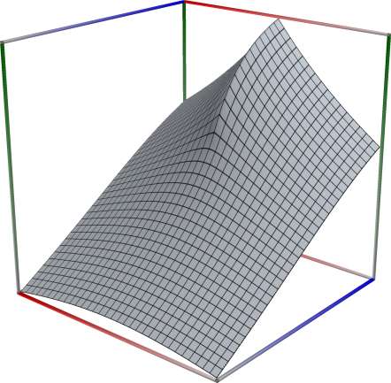
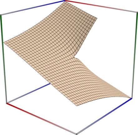
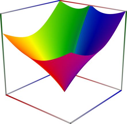
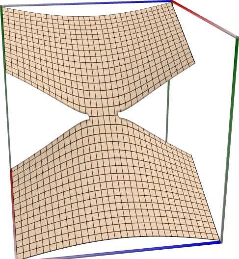
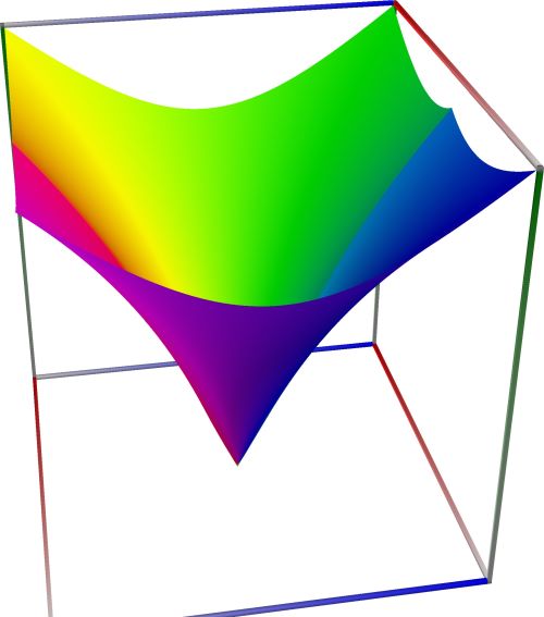
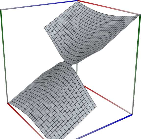
05a_TestPolylog_re \(\quad\) 05b_TestPolylog_im \(\quad\) 05c_TestPolylog_abs

Left figure: real part of the Polylogarithm, \(\mathrm{Li}_s(z)\). Camera angles are \(\theta=135^\circ\) and \(\phi = -12^\circ\), camera radius is -2.

Middle figure: imaginary part of the Polylogarithm, \(\mathrm{Li}_s(z)\). Camera angles are \(\theta=135^\circ\) and \(\phi = -12^\circ\), camera radius is -2.

Right figure: absolute value of the Polylogarithm, \(\mathrm{Li}_s(z)\), with color-coded phase. Camera angles are \(\theta=135^\circ\) and \(\phi = -12^\circ\), camera radius is -2.

An example in Python

>>> from xlcalcnet import xreal
>>> xreal.PolylogR(2, 0.5)
xreal('5.2359877559829887307E-1')
>>> xreal.PolylogR(2, '0.1')
xreal('5.3518479027559984754E-1')

An example in Visual Basic

>>> from xlcalcnet import Gpr
>>> Gpr.PolylogR(2, 0.5)
Gpr('5.2359877559829887307E-1')
>>> Gpr.PolylogR(2, '0.1')
Gpr('5.3518479027559984754E-1')

An example with real input:

>>> from xlcalcnet import dec, mpm, gmp, fpm, apm
>>> mpm.dps = 40; s = '10'; x = '0.5'
>>> \mathrm{d}x = dec.polylog(s, x); mx = mpm.polylog(s, x); gx = gmp.polylog(s, x)
>>> fx = fpm.polylog(s, x); ax = apm.polylog(s, x)
>>> mpm.show([\mathrm{d}x, mx, gx, fx, ax])
dec:  5.002463206060067750096752404960275553344E-1
mpm:  5.002463206060067750096752404960275553344e-1
gmp:  5.002463206060067750096752404960275553344E-01
fpm:  5.00246320606007E-01
apm:  5.002463206060067750096752404756715463182e-1 (4.658e-24%)

An example with complex input:

>>> from xlcalcnet import dec, mpm, gmp, fpm, apm
>>> mpm.dps = 20; s = '10'; z = '5.0 + 3j'
>>> \mathrm{d}z = dec.polylog(s, z); mz = mpm.polylog(s, z); gz = gmp.polylog(m, z)
>>> fz = fpm.polylog(m, z); az = apm.polylog(m, z)
>>> mpm.show([\mathrm{d}z, mz, gz, fz, az],  aligned=True)
dec: 5.0140954368998825423E+0             + 3.0330881889981661901E+0j
mpm: 5.0140954368998825423e+0             + 3.0330881889981661901e+0j
gmp: 5.0140954368998825423E+00            + 3.0330881889981661901E+00j
fpm: 5.01409543689988E+00                 + 3.03308818899817E+00j
apm: 5.0140954366116116588e+0 (1.145e-5%) + 3.0330881892210954918e+0 (2.687e-5%)j

Trilogarithm Function, \(\mathrm{Li}_3(z)\)#

math53.trilog(x)#

Returns the trilogarithm \(\displaystyle \mathrm{trilog}(x) = \Re \displaystyle \mathrm{Li}_3(x)\). See also Wikipedia [1442], MathWorld [1028], NIST [17], Ehrhardt [309] (3.6.14), Mpmath [692].

An example in Python

>>> from xlcalcnet import xreal
>>> xreal.Trilog(0.5)
xreal('5.2359877559829887307E-1')
>>> xreal.Trilog('0.1')
xreal('5.3518479027559984754E-1')

An example in Visual Basic

>>> from xlcalcnet import Gpr
>>> Gpr.Trilog(0.5)
Gpr('5.2359877559829887307E-1')
>>> Gpr.Trilog('0.1')
Gpr('5.3518479027559984754E-1')

Dilogarithm Function, \(\mathrm{Li}_2(z)\)#

ctx.dilog(x)#

where ctx is math53, mathc53 or ctxflint.

Returns the dilogarithm \(\displaystyle \mathrm{dilog}(x) = \Re \displaystyle \mathrm{Li}_2(x) = -\Re \int_0^x \frac{\log(1-t)}{t} \, \mathrm{d}t\).

See also Wikipedia [1442], MathWorld [1028], NIST [17], Ehrhardt [309] (3.6.13), Ehrhardt [309] (4.2.25), Flint [840], Mpmath [692].

This function returns the dilogarithm function

\[\text{dilog}(x) = \Re \text{Li}_2(x) = -\Re \int_0^x \frac{\log(1-t)}{t}\mathrm{d}t.\]

Note that there is some confusion about the naming: some authors and/or computer algebra systems use \(\text{dilog}(x) = \text{Li}_2(1-x)\) and then call \(\text{Li}_2(x)\) Spence function/integral or similar.
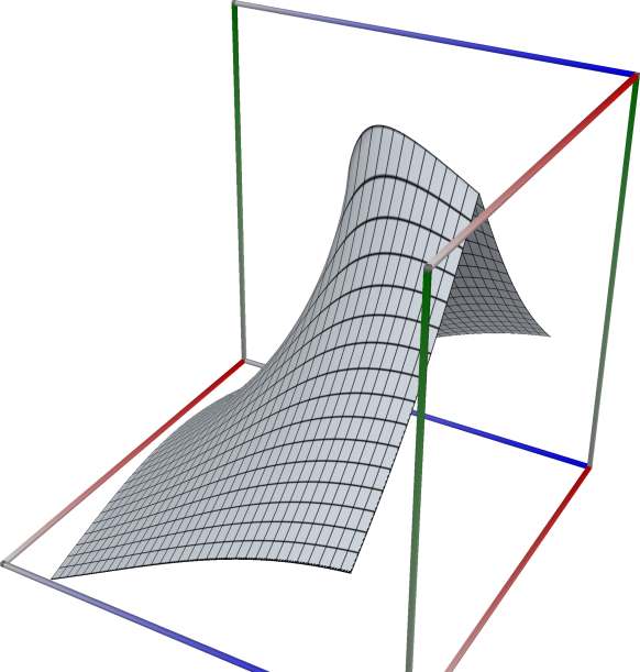
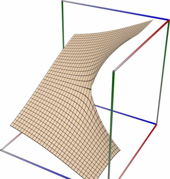
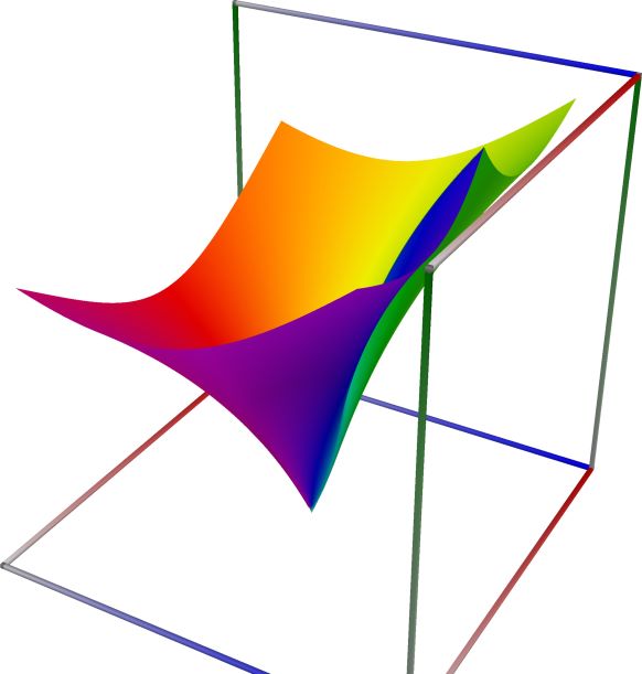
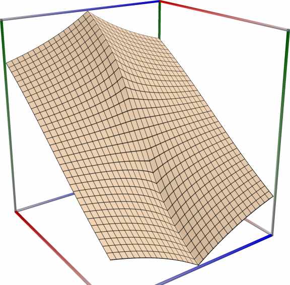
06a_TestDilog_re \(\quad\) 06b_TestDilog_im \(\quad\) 06c_TestDilog_abs

Left figure: real part of the Dilog function, \(\mathrm{Li}_2(z)\). Camera angles are \(\theta=135^\circ\) and \(\phi = -12^\circ\), camera radius is -2.

Middle figure: imaginary part of the Dilog function, \(\mathrm{Li}_2(z)\). Camera angles are \(\theta=135^\circ\) and \(\phi = -12^\circ\), camera radius is -2.

Right figure: absolute value of the Dilog function, \(\mathrm{Li}_2(z)\), with color-coded phase. Camera angles are \(\theta=135^\circ\) and \(\phi = -12^\circ\), camera radius is -2.

An example in Python

>>> from xlcalcnet import xreal
>>> xreal.Dilog(0.5)
xreal('5.2359877559829887307E-1')
>>> xreal.Dilog('0.1')
xreal('5.3518479027559984754E-1')

An example in Visual Basic

>>> from xlcalcnet import Gpr
>>> Gpr.Dilog(0.5)
Gpr('5.2359877559829887307E-1')
>>> Gpr.Dilog('0.1')
Gpr('5.3518479027559984754E-1')

An example with real input:

>>> from xlcalcnet import dec, mpm, gmp, fpm, apm
>>> mpm.dps = 40; x = '0.5'
>>> \mathrm{d}x = dec.dilog(x); mx = mpm.dilog(x); gx = gmp.dilog(x)
>>> fx = fpm.dilog(x); ax = apm.dilog(x)
>>> mpm.show([\mathrm{d}x, mx, gx, fx, ax])
dec:  5.822405264650125059026563201596801087442E-1
mpm:  5.822405264650125059026563201596801087442e-1
gmp:  5.822405264650125059026563201596801087442E-01
fpm:  5.82240526465013E-01
apm:  5.822405264650125059026563201596801087442e-1 (9.858e-40%)

An example with complex input:

>>> from xlcalcnet import dec, mpm, gmp, fpm, apm
>>> mpm.dps = 20; z = '5.0 + 3j'
>>> \mathrm{d}z = dec.dilog(z); mz = mpm.dilog(z); gz = gmp.dilog(z)
>>> fz = fpm.dilog(z); az = apm.dilog(z)
>>> mpm.show([\mathrm{d}z, mz, gz, fz, az],  aligned=True)
dec: 3.3260008208192192025E-2              + 4.6816673723804519905E+0j
mpm: 3.3260008208192192025e-2              + 4.6816673723804519905e+0j
gmp: 3.3260008208192192025E-02             + 4.6816673723804519905E+00j
fpm: 3.32600082081922E-02                  + 4.68166737238045E+00j
apm: 3.3260008208192192025e-2 (7.958e-20%) + 4.6816673723804519905e+0 (7.237e-20%)j

Generalized Clausen sine function#

ctxflint.clausen_sin(s, z)#

Returns the Clausen sine function. See also Wikipedia [1465], MathWorld [1095], Mpmath [737].

Computes the Clausen sine function, defined formally by the series

\[\mathrm{Cl}_s(z) = \sum_{k=1}^{\infty} \frac{\sin(kz)}{k^s}.\]

The special case \(\mathrm{Cl}_2(z)\) (i.e. clsin(2,z)) is the classical “Clausen function”. More generally, the Clausen function is defined for complex \(s\) and \(z\), even when the series does not converge. The Clausen function is related to the polylogarithm (polylog()) as

\[ \begin{align}\begin{aligned}\mathrm{Cl}_s(z) = \frac{1}{2i}\left(\mathrm{Li}_s\left(e^{iz}\right) - \mathrm{Li}_s\left(e^{-iz}\right)\right)\\= \mathrm{Im}\left[\mathrm{Li}_s(e^{iz})\right] \quad (s, z \in \mathbb{R}),\end{aligned}\end{align} \]

and this representation can be taken to provide the analytic continuation of the series. The complementary function clcos() gives the corresponding cosine sum.
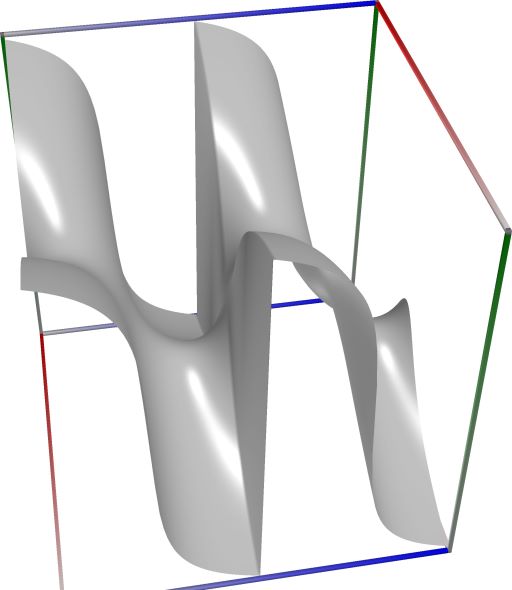
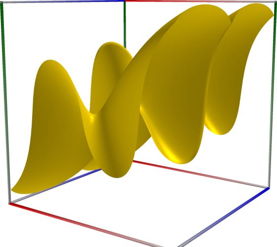
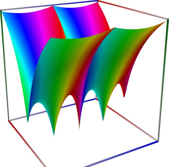
07a_TestClausenSin_re \(\quad\) 07b_TestClausenSin_im \(\quad\) 07c_TestClausenSin_abs

Left figure: real part of the Generalized Clausen sine function. Camera angles are \(\theta=135^\circ\) and \(\phi = -12^\circ\), camera radius is -2.

Middle figure: imaginary part of the Generalized Clausen sine function. Camera angles are \(\theta=135^\circ\) and \(\phi = -12^\circ\), camera radius is -2.

Right figure: absolute value of the Generalized Clausen sine function, with color-coded phase. Camera angles are \(\theta=135^\circ\) and \(\phi = -12^\circ\), camera radius is -2.

An example with real input:

>>> from xlcalcnet import dec, mpm, gmp, fpm, apm
>>> mpm.dps = 40; s = '3'; x = '4'
>>> \mathrm{d}x = dec.clsin(s, x); mx = mpm.clsin(s, x); gx = gmp.clsin(s, x)
>>> fx = fpm.clsin(s, x); ax = apm.clsin(s, x)
>>> mpm.show([\mathrm{d}x, mx, gx, fx, ax])
dec:  -6.533010136329338746275795332005774465795E-1
mpm:  -6.533010136329338746275795332005774465795e-1
gmp:  -6.533010136329338746275795332005774465795E-01
fpm:  -6.53301013632934E-01
apm:  -6.533010136329338746275795332005774886000e-1 (-2.242e-29%)

An example with complex input:

>>> from xlcalcnet import dec, mpm, gmp, fpm, apm
>>> mpm.dps = 20; s = '3'; z = '5.0 + 3j'
>>> \mathrm{d}z = dec.clsin(s, z); mz = mpm.clsin(s, z); gz = gmp.clsin(s, z)
>>> fz = fpm.clsin(s, z); az = apm.clsin(s, z)
>>> mpm.show([\mathrm{d}z, mz, gz, fz, az],  aligned=True)
dec: -5.1750336134513741048E+0               - 2.1271427013787699791E+0j
mpm: -5.1750336134513741048e+0               - 2.1271427013787699791e+0j
gmp: -5.1750336134513741048E+00              - 2.1271427013787699791E+00j
fpm: -5.17503361345137E+00                   - 2.12714270137877E+00j
apm: -5.1750336134513741059e+0 (-3.604e-14%) - 2.1271427013787699777e+0 (-7.287e-14%)j

Generalized Clausen cosine function#

ctxflint.clausen_cos(s, z)#

Returns the Clausen cosine function. See also Wikipedia [1465], MathWorld [1095], Mpmath [736].

Computes the Clausen cosine function, defined formally by the series

\[\mathrm{\widetilde{Cl}}_s(z) = \sum_{k=1}^{\infty} \frac{\cos(kz)}{k^s}.\]

This function is complementary to the Clausen sine function clsin(). In terms of the polylogarithm,

\[ \begin{align}\begin{aligned}\mathrm{\widetilde{Cl}}_s(z) = \frac{1}{2}\left(\mathrm{Li}_s\left(e^{iz}\right) + \mathrm{Li}_s\left(e^{-iz}\right)\right)\\= \mathrm{Re}\left[\mathrm{Li}_s(e^{iz})\right] \quad (s, z \in \mathbb{R}).\end{aligned}\end{align} \]
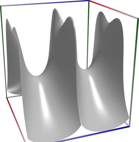
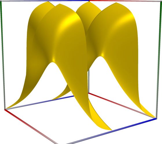
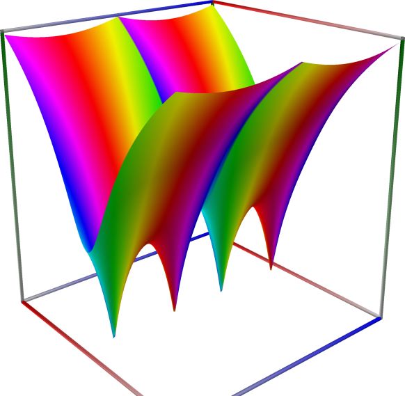
08a_TestClausenCos_re \(\quad\) 08b_TestClausenCos_im \(\quad\) 08c_TestClausenCos_abs

Left figure: real part of the Generalized Clausen cosine function. Camera angles are \(\theta=135^\circ\) and \(\phi = -12^\circ\), camera radius is -2.

Middle figure: imaginary part of the Generalized Clausen cosine function. Camera angles are \(\theta=135^\circ\) and \(\phi = -12^\circ\), camera radius is -2.

Right figure: absolute value of the Generalized Clausen cosine function, with color-coded phase. Camera angles are \(\theta=135^\circ\) and \(\phi = -12^\circ\), camera radius is -2.

An example with real input:

>>> from xlcalcnet import dec, mpm, gmp, fpm, apm
>>> mpm.dps = 40; s = '3'; x = '4'
>>> \mathrm{d}x = dec.clcos(s, x); mx = mpm.clcos(s, x); gx = gmp.clcos(s, x)
>>> fx = fpm.clcos(s, x); ax = apm.clcos(s, x)
>>> mpm.show([\mathrm{d}x, mx, gx, fx, ax])
dec:  -6.518926267198991308332758909517770104595E-1
mpm:  -6.518926267198991308332758909517770104595e-1
gmp:  -6.518926267198991308332758909517770104595E-01
fpm:  -6.51892626719899E-01
apm:  -6.518926267198991308332758909517763900500e-1 (-5.188e-29%)

An example with complex input:

>>> from xlcalcnet import dec, mpm, gmp, fpm, apm
>>> mpm.dps = 20; s = '3'; z = '5.0 + 3j'
>>> \mathrm{d}z = dec.clcos(s, z); mz = mpm.clcos(s, z); gz = gmp.clcos(s, z)
>>> fz = fpm.clcos(s, z); az = apm.clcos(s, z)
>>> mpm.show([\mathrm{d}z, mz, gz, fz, az],  aligned=True)
dec: -2.1132834047743479436E+0               + 5.1271260828837504331E+0j
mpm: -2.1132834047743479436e+0               + 5.1271260828837504331e+0j
gmp: -2.1132834047743479436E+00              + 5.1271260828837504331E+00j
fpm: -2.11328340477435E+00                   + 5.12712608288375E+00j
apm: -2.1132834047743479423e+0 (-7.335e-14%) + 5.1271260828837504341e+0 (3.638e-14%)j

Classical Clausen function, \(\mathrm{Cl}_2(x)\)#

math53.clausen2(x)#

Returns the Clausen function \(\displaystyle \mathrm{Cl}_2(x) = \Im \displaystyle \mathrm{Li}_2(e^{ix}) = \int_0^x \log|2\sin(t/2)| \, \mathrm{d}t\).

See also: Wikipedia [1465], MathWorld [1095], Ehrhardt [309] (3.6.15), Mpmath [736].

An example in Python

>>> from xlcalcnet import xreal
>>> xreal.Clausen2(0.5)
xreal('5.2359877559829887307E-1')
>>> xreal.Clausen2('0.1')
xreal('5.3518479027559984754E-1')

An example in Visual Basic

>>> from xlcalcnet import Gpr
>>> Gpr.Clausen2(0.5)
Gpr('5.2359877559829887307E-1')
>>> Gpr.Clausen2('0.1')
Gpr('5.3518479027559984754E-1')

Bose-Einstein integrals, \(G_s(x)\)#

math53.bose_einstein(s, x)#

Returns the Bose-Einstein integral of real order \(s\), \(\displaystyle G_s(x) = \frac{1}{\Gamma(s+1)} \int_0^{\infty} \frac{t^s}{e^{t-x}-1} = \text{Li}_{s+1}(e^x) \,\). If \(x>0\) the real part of \(G_s(x)\) is returned.

See also: MathWorld [1024], Ehrhardt [309] (3.6.7), NIST [16].

\[G_{s}(x)=\frac{1}{\Gamma\left(s+1\right)}\int_{0}^{\infty}\frac{t^{s}}{e^{t-x}-1}\mathrm{d}t,\]

In terms of polylogarithms:

\[G_{s}(x)=\mathrm{Li}_{s+1}\left(e^{x}\right).\]

An example in Python

>>> from xlcalcnet import xreal
>>> xreal.BoseEinstein(2,5)
xreal('5.2359877559829887307E-1')
>>> xreal.BoseEinstein(2,'51')
xreal('5.3518479027559984754E-1')

An example in Visual Basic

>>> from xlcalcnet import Gpr
>>> Gpr.BoseEinstein(2,5)
Gpr('5.2359877559829887307E-1')
>>> Gpr.BoseEinstein(2,'51')
Gpr('5.3518479027559984754E-1')

An example with real input:

>>> from xlcalcnet import dec, mpm, gmp, fpm, apm
>>> mpm.dps = 40; s = '10'; x = '0.5'
>>> \mathrm{d}x = dec.bose_einstein(s, x); mx = mpm.bose_einstein(s, x); gx = gmp.bose_einstein(s, x)
>>> fx = fpm.bose_einstein(s, x); ax = apm.bose_einstein(s, x)
>>> mpm.show([\mathrm{d}x, mx, gx, fx, ax])
dec:  1.650075952950667128565820621131669931198E+0
mpm:  1.650075952950667128565820621131669931198e+0
gmp:  1.650075952950667128565820621131669931198E+00
fpm:  1.65007595295067E+00
apm:  1.650075952950667128565820642266282738366e+0 (2.139e-21%)

An example with complex input:

>>> from xlcalcnet import dec, mpm, gmp, fpm, apm
>>> mpm.dps = 20; s = '10'; z = '5.0 + 3j'
>>> \mathrm{d}z = dec.bose_einstein(s, z); mz = mpm.bose_einstein(s, z); gz = gmp.bose_einstein(s, z)
>>> fz = fpm.bose_einstein(s, z); az = apm.bose_einstein(s, z)
>>> mpm.show([\mathrm{d}z, mz, gz, fz, az],  aligned=True)
dec: -1.4096051587148306166E+2             + 1.9476656215692471738E+1j
mpm: -1.4096051587148306166e+2             + 1.9476656215692471738e+1j
gmp: -1.4096051587148306166E+02            + 1.9476656215692471738E+01j
fpm: -1.40960515871483E+02                 + 1.94766562156925E+01j
apm: -1.4096051581016388546e+2 (-7.08e-5%) + 1.9476656215507044363e+1 (0.0007137%)j

Fermi-Dirac integrals, \(F_s(x)\)#

ctx.fermi_dirac(s, x)#

where ctx is math53 or ctxflint.

Returns the Fermi-Dirac integral of order \(s\), \(\displaystyle F_s(x) = \frac{1}{\Gamma(s+1)} \int_0^{\infty} \frac{t^s}{e^{t-x}+1} = -\text{Li}_{s+1}(-e^x) \,\).

See also: Wikipedia [1425], MathWorld [1030], Ehrhardt [309] (3.6.8.1).

\[F_{s}(x)=\frac{1}{\Gamma\left(s+1\right)}\int_{0}^{\infty}\frac{t^{s}}{e^{t-x}+1}\mathrm{d}t,\]

\(F_{s}(x)=-\mathrm{Li}_{s+1}\left(-e^{x}\right),\)

An example in Python

>>> from xlcalcnet import xreal
>>> xreal.FermiDiracR(2,5)
xreal('5.2359877559829887307E-1')
>>> xreal.FermiDiracR(2,'51')
xreal('5.3518479027559984754E-1')

An example in Visual Basic

>>> from xlcalcnet import Gpr
>>> Gpr.FermiDiracR(2,5)
Gpr('5.2359877559829887307E-1')
>>> Gpr.FermiDiracR(2,'51')
Gpr('5.3518479027559984754E-1')

An example with real input:

>>> from xlcalcnet import dec, mpm, gmp, fpm, apm
>>> mpm.dps = 40; s = '10'; x = '1.5'
>>> \mathrm{d}x = dec.fermi_dirac(s, x); mx = mpm.fermi_dirac(s, x); gx = gmp.fermi_dirac(s, x)
>>> fx = fpm.fermi_dirac(s, x); ax = apm.fermi_dirac(s, x)
>>> mpm.show([\mathrm{d}x, mx, gx, fx, ax])
dec:  4.472317812068368662350774526763653861048E+0
mpm:  4.472317812068368662350774526763653861048e+0
gmp:  4.472317812068368662350774526763653861048E+00
fpm:  4.47231781206837E+00
apm:  4.472317812068368662350774520946064383782e+0 (1.711e-22%)

An example with complex input:

>>> from xlcalcnet import dec, mpm, gmp, fpm, apm
>>> mpm.dps = 20; s = '10'; z = '5.0 + 3j'
>>> \mathrm{d}z = dec.fermi_dirac(s, z); mz = mpm.fermi_dirac(s, z); gz = gmp.fermi_dirac(s, z)
>>> fz = fpm.fermi_dirac(s, z); az = apm.fermi_dirac(s, z)
>>> mpm.show([\mathrm{d}z, mz, gz, fz, az],  aligned=True)
dec: -1.5096075557263597965E+2              + 3.0204317063642472857E+1j
mpm: -1.5096075557263597965e+2              + 3.0204317063642472857e+1j
gmp: -1.5096075557263597965E+02             + 3.0204317063642472857E+01j
fpm: -1.50960755572636E+02                  + 3.02043170636425E+01j
apm: -1.5096075564796857312e+2 (-7.353e-5%) + 3.0204317086095309026e+1 (0.0004834%)j

Legendre’s Chi function, \(\chi_s(x)\)#

math53.legendre_chi(s, x)#

Returns Legendre’s Chi function, defined as \(\displaystyle \chi_s(x) = \sum_{n=0}^{\infty} \frac{x^{2n+1}}{(2n+1)^s} = \tfrac{1}{2} \left( \text{Li}_s(x) - \text{Li}_s(-x) \right) \,\), for \(s\ge 0, |x|\le 1\).

See also: Wikipedia [1434], MathWorld [1041], Ehrhardt [309] (3.6.9).

The function can be expressed as

\[\chi_s(x)=2^{-s} x \Phi\left(x^2,s,\tfrac{1}{2}\right) = \tfrac{1}{2}\left(\text{Li}_s(x)-\text{Li}_s(-x) \right).\]

For large \(s > 22.8\) the function adds up to three terms of the sum, for \(s = 0\) or \(s = 1\) the \(Li_s\) relation is used, otherwise the result is computed with Lerch’s transcendent.
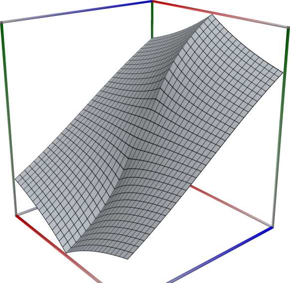
09a_TestLegendreChi_re \(\quad\) 09b_TestLegendreChi_im \(\quad\) 09c_TestLegendreChi_abs

Left figure: real part of Legendre’s Chi function, \(\chi_s(x)\). Camera angles are \(\theta=135^\circ\) and \(\phi = -12^\circ\), camera radius is -2.

Middle figure: imaginary part of Legendre’s Chi function, \(\chi_s(x)\). Camera angles are \(\theta=135^\circ\) and \(\phi = -12^\circ\), camera radius is -2.

Right figure: absolute value of Legendre’s Chi function, \(\chi_s(x)\), with color-coded phase. Camera angles are \(\theta=135^\circ\) and \(\phi = -12^\circ\), camera radius is -2.

An example in Python

>>> from xlcalcnet import xreal
>>> xreal.LegendreChi(2,5, 0.5)
xreal('5.2359877559829887307E-1')
>>> xreal.LegendreChi('5.1', 0.5)
xreal('5.3518479027559984754E-1')

An example in Visual Basic

>>> from xlcalcnet import Gpr
>>> Gpr.LegendreChi(2,5, 0.5)
Gpr('5.2359877559829887307E-1')
>>> Gpr.LegendreChi('5.1', 0.5)
Gpr('5.3518479027559984754E-1')

An example with real input:

>>> from xlcalcnet import dec, mpm, gmp, fpm, apm
>>> mpm.dps = 40; s = '10'; x = '1.5'
>>> \mathrm{d}x = dec.legendre_chi(s, x); mx = mpm.legendre_chi(s, x); gx = gmp.legendre_chi(s, x)
>>> fx = fpm.legendre_chi(s, x); ax = apm.legendre_chi(s, x)
>>> mpm.show([\mathrm{d}x, mx, gx, fx, ax])
dec:  1.500058011828613644574663245595439676243E+0
mpm:  1.500058011828613644574663245595439676243e+0
gmp:  1.500058011828613644574663245595439676243E+00
fpm:  1.50005801182861E+00
apm:  1.500058011828613644574663246586459327124e+0 (2.88e-22%)

An example with complex input:

>>> from xlcalcnet import dec, mpm, gmp, fpm, apm
>>> mpm.dps = 20; s = '10'; z = '5.0 + 3j'
>>> \mathrm{d}z = dec.legendre_chi(s, z); mz = mpm.legendre_chi(s, z); gz = gmp.legendre_chi(s, z)
>>> fz = fpm.legendre_chi(s, z); az = apm.legendre_chi(s, z)
>>> mpm.show([\mathrm{d}z, mz, gz, fz, az],  aligned=True)
dec: 4.9993028299912224901E+0             + 3.0032350570493713371E+0j
mpm: 4.9993028299912224901e+0             + 3.0032350570493713371e+0j
gmp: 4.9993028299912224901E+00            + 3.0032350570493713371E+00j
fpm: 4.99930282999122E+00                 + 3.00323505704937E+00j
apm: 4.9993028304470985305e+0 (2.364e-5%) + 3.0032350577905899996e+0 (4.62e-5%)j

Generalized inverse tangent integral#

ctxflint.inverse_tan_integral(s, z)#

Returns the generalized inverse tangent integral \(Ti_s(z)\).

See also: Wikipedia [1439], MathWorld [1037].

This function returns the inverse-tangent integral

\[\text{Ti}_2(x) = \int_0^x \frac{\arctan(t)}{t} \mathrm{d}t.\]

For \(x>1\) the relation

\[\text{Ti}_2(x) = \text{Ti}_2\left(\frac{1}{x}\right) + \frac{\pi}{2} \log(x)\]

is used, and for \(x<0\) the result is \(\text{Ti}_2(x) = -\text{Ti}_2(-x)\).

See also MathWorld

The inverse tangent integral Tis(z) (Lewin 1958, Ch. VII § 1.2) can be expressed in terms of polylogarithms:

\[\mathrm {Ti} _{s}(z)={1 \over 2i}\left[\mathrm {Li} _{s}(iz)-\mathrm {Li} _{s}(-iz)\right].\]

The relation in particular implies:

\[\mathrm {Ti} _{0}(z)={z \over 1+z^{2}},\quad \mathrm {Ti} _{1}(z)=\arctan z,\quad \mathrm {Ti} _{2}(z)=\int _{0}^{z}{\arctan t \over t}\mathrm{d}t,\quad \ldots ~\quad \mathrm {Ti} _{n+1}(z)=\int _{0}^{z}{\frac {\mathrm {Ti} _{n}(t)}{t}}\mathrm{d}t,\]

which explains the function name.

10a_TestTangentInt_re \(\quad\) 10b_TestTangentInt_im \(\quad\) 10c_TestTangentInt_abs

Left figure: real part of the Generalized inverse tangent integral. Camera angles are \(\theta=135^\circ\) and \(\phi = -12^\circ\), camera radius is -2.

Middle figure: imaginary part of the Generalized inverse tangent integral. Camera angles are \(\theta=135^\circ\) and \(\phi = -12^\circ\), camera radius is -2.

Right figure: absolute value of the Generalized inverse tangent integral, with color-coded phase. Camera angles are \(\theta=135^\circ\) and \(\phi = -12^\circ\), camera radius is -2.

An example with real input:

>>> from xlcalcnet import dec, mpm, gmp, fpm, apm
>>> mpm.dps = 40; s = '10'; x = '1.5'
>>> \mathrm{d}x = dec.ti(s, x); mx = mpm.ti(s, x); gx = gmp.ti(s, x)
>>> fx = fpm.ti(s, x); ax = apm.ti(s, x)
>>> mpm.show([\mathrm{d}x, mx, gx, fx, ax])
dec:  1.499943569822004012305079650116043572538E+0
mpm:  1.499943569822004012305079650116043572538e+0
gmp:  1.499943569822004012305079650116043572538E+00
fpm:  1.49994356982200E+00
apm:  1.499943569822004012305079649905189176482e+0 (9.317e-24%)

An example with complex input:

>>> from xlcalcnet import dec, mpm, gmp, fpm, apm
>>> mpm.dps = 20; s = '10'; z = '5.0 + 3j'
>>> \mathrm{d}z = dec.ti(s, z); mz = mpm.ti(s, z); gz = gmp.ti(s, z)
>>> fz = fpm.ti(s, z); az = apm.ti(s, z)
>>> mpm.show([\mathrm{d}z, mz, gz, fz, az],  aligned=True)
dec: 4.9998641623415218366E+0             + 2.9969552556663645569E+0j
mpm: 4.9998641623415218366e+0             + 2.9969552556663645569e+0j
gmp: 4.9998641623415218366E+00            + 2.9969552556663645569E+00j
fpm: 4.99986416234152E+00                 + 2.99695525566636E+00j
apm: 4.9998641636149685969e+0 (3.517e-5%) + 2.9969552549261524848e+0 (4.218e-5%)j
math53.tangent_int(s, x)#

Returns the inverse tangent integral of real order \(s\), \(\displaystyle \mathrm{Ti}_s(x) = \sum_{k=0}^{\infty} \frac{(-1)^k x^{2k+1}}{(2k+1)^s}, \quad |x|<1\).

See also: Wikipedia [1439], MathWorld [1037], Ehrhardt [309] (3.6.17).

An example in Python

>>> from xlcalcnet import xreal
>>> xreal.TangentInt2(2,0.5)
xreal('5.2359877559829887307E-1')
>>> xreal.TangentInt2(2,'0.1')
xreal('5.3518479027559984754E-1')

An example in Visual Basic

>>> from xlcalcnet import Gpr
>>> Gpr.TangentInt2(2,0.5)
Gpr('5.2359877559829887307E-1')
>>> Gpr.TangentInt2(2,'0.1')
Gpr('5.3518479027559984754E-1')

previous

Polygamma and related functions

next

Hurwitz zeta and related functions

Contents
  • Polylogarithm, \(\mathrm{Li}_s(z)\)
    • ctx.polylog()
  • Trilogarithm Function, \(\mathrm{Li}_3(z)\)
    • math53.trilog()
  • Dilogarithm Function, \(\mathrm{Li}_2(z)\)
    • ctx.dilog()
  • Generalized Clausen sine function
    • ctxflint.clausen_sin()
  • Generalized Clausen cosine function
    • ctxflint.clausen_cos()
  • Classical Clausen function, \(\mathrm{Cl}_2(x)\)
    • math53.clausen2()
  • Bose-Einstein integrals, \(G_s(x)\)
    • math53.bose_einstein()
  • Fermi-Dirac integrals, \(F_s(x)\)
    • ctx.fermi_dirac()
  • Legendre’s Chi function, \(\chi_s(x)\)
    • math53.legendre_chi()
  • Generalized inverse tangent integral
    • ctxflint.inverse_tan_integral()
    • math53.tangent_int()

By Dietrich Hadler

© Copyright 2026, Dietrich Hadler. .

Last updated on Aug 19, 2026.