Hypergeometric Limit Function \(\,_0F_1\)#

Confluent Hypergeometric Limit Function \({}_0F_1(b,x)\)#

ctx.hyperg_0f1(b, x)#

Returns \(\displaystyle {}_0F_1(b,x) = \sum_{k=0}^{\infty} \frac{1}{(b)_k} \frac{x^k}{k!}\), the confluent hypergeometric limit function, where \(b \ne 0,-1,-2,\ldots\)

See also Wikipedia [1360], MathWorld [974] BoostMath [110], Ehrhardt [309] (3.8.6), Flint [823], Flint [816], Mpmath [618].

If ctx is math53, ctxboost or ctxflintreal, then \(b, x \in \mathbb{R}\) is exspected. If ctx is cmath53, then \(b \in \mathbb{R}\) and \(x \in \mathbb{C}\) is exspected. If ctx is ctxflintcplx then \(b, x \in \mathbb{C}\) is accepted.

Calls arb_hypgeom_0f1 or acb_hypgeom_0f1.

Returns the hypergeometric function \({}_0F_1\).

Gives the hypergeometric function \({}_0F_1\), sometimes known as the confluent limit function, defined as

\[{}_0F_1(a,z) = \sum_{k=0}^{\infty} \frac{1}{(a)_k} \frac{z^k}{k!}.\]

\(\quad\) \(\quad\)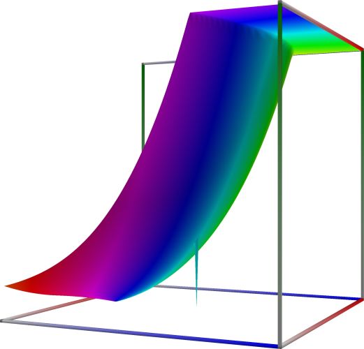

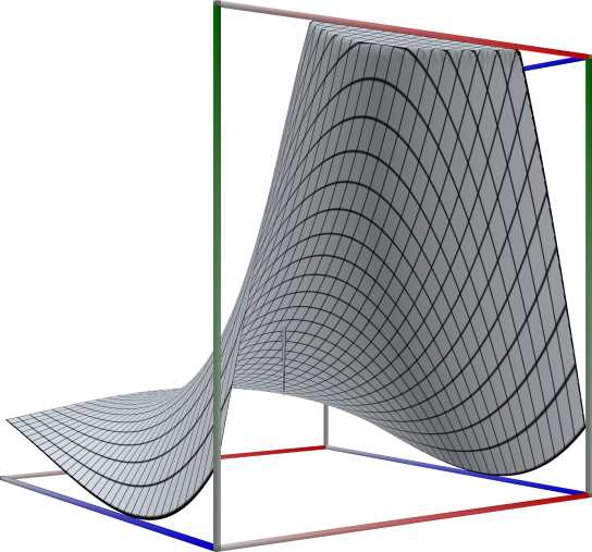
Left figure: real part of the Hypergeometric function \({}_0F_1\). Camera angles are \(\theta=135^\circ\) and \(\phi = -12^\circ\), camera radius is -2.

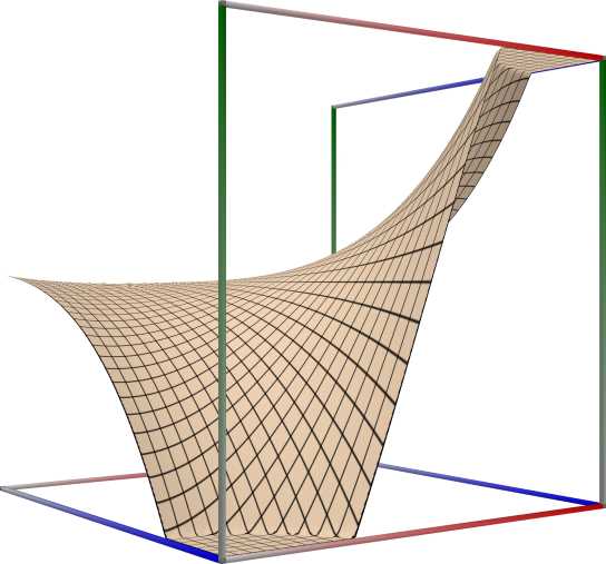
Middle figure: imaginary part of the Hypergeometric function \({}_0F_1\). Camera angles are \(\theta=135^\circ\) and \(\phi = -12^\circ\), camera radius is -2.

Right figure: absolute value of the Hypergeometric function \({}_0F_1\), with color-coded phase. Camera angles are \(\theta=135^\circ\) and \(\phi = -12^\circ\), camera radius is -2.

An example in Python

>>> from xlcalcnet import xreal
>>> xreal.Hyperg0F1(5.1,0.5)
xreal('5.2359877559829887307E-1')
>>> xreal.Hyperg0F1(15.2,0.5)
xreal('5.3518479027559984754E-1')

An example in Visual Basic

>>> from xlcalcnet import Gpr
>>> Gpr.Hyperg0F1(5.1,0.5)
Gpr('5.2359877559829887307E-1')
>>> Gpr.Hyperg0F1(15.2,0.5)
Gpr('5.3518479027559984754E-1')

An example with real input:

>>> from xlcalcnet import dec, mpm, gmp, fpm, apm
>>> mpm.dps = 40; a= 10; x = 30
>>> \mathrm{d}x = dec.hyp0f1(a, x); mx = mpm.hyp0f1(a, x); gx = gmp.hyp0f1(a, x)
>>> fx = fpm.hyp0f1(a, x); ax = apm.hyp0f1(a, x)
>>> mpm.show([\mathrm{d}x, mx, gx, fx, ax])
dec:  1.468615500968110064708314782694224995260E+1
mpm:  1.468615500968110064708314782694224995260e+1
gmp:  1.468615500968110064708314782694224995260E+01
fpm:  1.46861550096811E+01
apm:  1.468615500968110064708314782694224995260e+1 (1.251e-39%)

An example with complex input:

>>> from xlcalcnet import dec, mpm, gmp, fpm, apm
>>> mpm.dps = 20; a= 10; z = '3 + 4j'
>>> \mathrm{d}z = dec.hyp0f1(a, z); mz = mpm.hyp0f1(a, z); gz = gmp.hyp0f1(a, z)
>>> fz = fpm.hyp0f1(a, z); az = apm.hyp0f1(a, z)
>>> mpm.show([\mathrm{d}z, mz, gz, fz, az],  aligned=True)
dec: 1.2521260436915235828E+0              + 5.1371862393580499600E-1j
mpm: 1.2521260436915235828e+0              + 5.1371862393580499600e-1j
gmp: 1.2521260436915235828E+00             + 5.1371862393580499600E-01j
fpm: 1.25212604369152E+00                  + 5.13718623935805E-01j
apm: 1.2521260436915235828e+0 (1.353e-19%) + 5.1371862393580499600e-1 (8.244e-20%)j

Regularized Confluent Hypergeometric Limit Function \({}_0\widetilde{F}_1(b;x)\)#

ctx.hyperg_0f1r(b, x)#

Returns \(\displaystyle {}_0\widetilde{F}_1(b;x) = \frac{1}{\Gamma(b)} {}_0F_1(b;x)\), the regularized confluent hypergeometric limit function, for \(b \ne 0, -1, -2, \cdots\), or, \(\\\) if \(b = 0, -1, -2, \cdots = -n\), the corresponding limit \(\displaystyle {}_0\widetilde{F}_1(b;x) = x^{n+1} {}_0\widetilde{F}_1(n+2;x) = \frac{x^{n+1}}{\Gamma(n+2)} {}_0F_1(n+2;x)\).

See also Wikipedia [1360], MathWorld [269] BoostMath [110], Ehrhardt [309] (3.8.7), Flint [823], Flint [816], Mpmath [618].