Gauss Hypergeometric Function \(\,_2F_1\)#

Gauss Hypergeometric Function, \({}_2F_1(a,b;c;x)\)#

ctx.hyperg_2f1(a, b, c, x)#

where ctx is math53 or ctxflint.

Note: math53.hyperg2F1(a, b, c, x)

Returns \(\displaystyle \,_2F_1(a,b,c,x) = \sum_{k=0}^{\infty} \frac{(a)_k (b)_k}{(c)_k} \frac{x^k}{k!}\), the Gauss hypergeometric function, defined for \(|x| < 1\).

See also Wikipedia [1365], MathWorld [969], NIST [199], Ehrhardt [309] (3.8.1), BoostMath [111], Flint [824], Flint [817], Mpmath [620].

Except for special cases it is required that \(-c \ne \mathbb{N}\). For \(x > 1\) the function is generally complex and not implemented in AMath; but if \(a\) or \(b\) is a non-positive integer, then \(\,_2F_1(a,b,c,x)\) becomes a polynomial in \(x\) and there is no restriction on \(x\).

Special values are \(\,_2F_1(0,b,c,x) = \,_2F_1(a,0,c,x) = \,_2F_1(a,b,c,0) = 1\) and, if \(c-a-b>0\), \(\displaystyle \,_2F_1(a,b,c,1) = \frac{\Gamma(c)\Gamma(c-a-b)}{\Gamma(c-a)\Gamma(c-b)}\).

In AMath the analytic continuation is done using one or two linear transformations: For all \(x < 1\) Abramowitz and Stegun. [4] equations (15.3.3-5) are used, and for \(0 < x < 1\) if \(c\) and \(c - a - b\) are no integers Abramowitz and Stegun. [4] equation (15.3.6). For \(c = a+b \pm m, (m = 0, 1, \ldots)\) the (complicated) formulas from Abramowitz and Stegun. [4] (15.3.10-12) are implemented. If \(a = -m\) is a negative integer (or \(b\) with \(a\) and \(b\) swapped, or both and \(a \ge b)\) the limiting cases for the (polynomial) transformations are implemented as in Abramowitz and Stegun. [4] equations (15.8.6/7).

This calls arb_hypgeom_2f1 or acb_hypgeom_2f1

Returns the Gauss hypergeometric function \({}_2F_1(a, b; c; z)\).

The Gauss hypergeometric function \({}_2F_1\) is defined for \(| z | < 1\) by the series

\[{}_2F_1(a,b;c;z) = \sum_{k=0}^\infty\frac{(a)_k(b)_k}{(c)_k}\cdot\frac{z^k}{k!}\]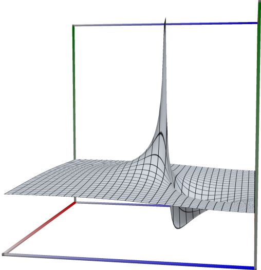

\(\quad\) \(\quad\)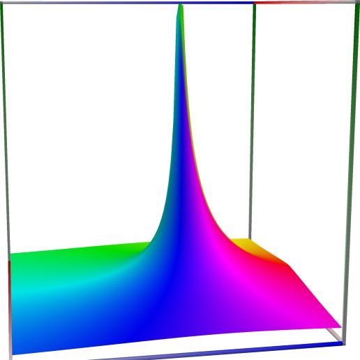

Left figure: real part of the Gauss Hypergeometric Function, \({}_2F_1(a,b;c;x)\). Camera angles are \(\theta=135^\circ\) and \(\phi = -12^\circ\), camera radius is -2.

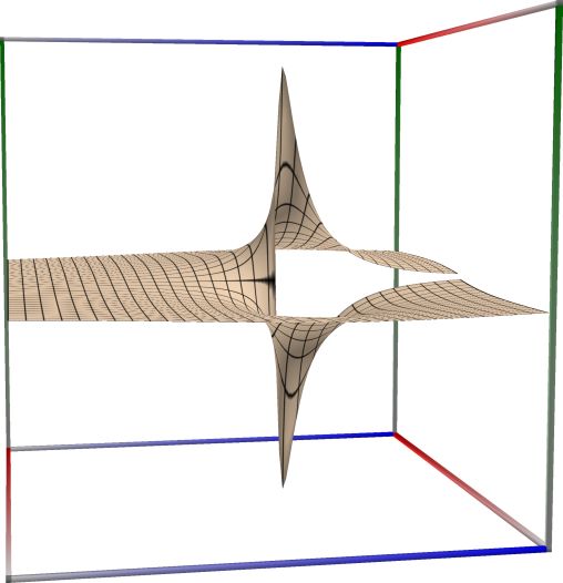
Middle figure: imaginary part of the Gauss Hypergeometric Function, \({}_2F_1(a,b;c;x)\). Camera angles are \(\theta=135^\circ\) and \(\phi = -12^\circ\), camera radius is -2.

Right figure: absolute value of the Gauss Hypergeometric Function, \({}_2F_1(a,b;c;x)\), with color-coded phase. Camera angles are \(\theta=135^\circ\) and \(\phi = -12^\circ\), camera radius is -2.

An example in Python

>>> from xlcalcnet import xreal
>>> xreal.Hyperg2F1(3,4,5,0.5)
xreal('5.2359877559829887307E-1')
>>> xreal.Hyperg2F1(13,14,15,0.5)
xreal('5.3518479027559984754E-1')

An example in Visual Basic

>>> from xlcalcnet import Gpr
>>> Gpr.Hyperg2F1(3,4,5,0.5)
Gpr('5.2359877559829887307E-1')
>>> Gpr.Hyperg2F1(13,14,15,0.5)
Gpr('5.3518479027559984754E-1')

An example with real input:

>>> from xlcalcnet import dec, mpm, gmp, fpm, apm
>>> mpm.dps = 40; a = '11.0'; b = '12.0'; c = '32.0'; x = '0.3'
>>> \mathrm{d}x = dec.hyp2f1(a, b, c, x); mx = mpm.hyp2f1(a, b, c, x); gx = gmp.hyp2f1(a, b, c, x)
>>> fx = fpm.hyp2f1(a, b, c, x); ax = apm.hyp2f1(a, b, c, x)
>>> mpm.show([\mathrm{d}x, mx, gx, fx, ax])
dec:  3.927580225263206566696488844725497448841E+0
mpm:  3.927580225263206566696488844725497448841e+0
gmp:  3.927580225263206566696488844725497448841E+00
fpm:  3.92758022526321E+00
apm:  3.927580225263206566696488844725497448841e+0 (2.338e-39%)

An example with complex input:

>>> from xlcalcnet import dec, mpm, gmp, fpm, apm
>>> mpm.dps = 20; a = '11.0 + 2.0j'; b = '12.0 + 3.0j'; c = '42.0 + 3.0j';z = '3.0 + 4.0j'
>>> \mathrm{d}z = dec.hyp2f1(a, b, c, z); mz = mpm.hyp2f1(a, b, c, z); gz = gmp.hyp2f1(a, b, c, z)
>>> fz = fpm.hyp2f1(a, b, c, z); az = apm.hyp2f1(a, b, c, z)
>>> mpm.show([\mathrm{d}z, mz, gz, fz, az], aligned=True)
dec: -1.0355451917135984282E-3              - 1.4654778601071805787E-3j
mpm: -1.0355451917135984282e-3              - 1.4654778601071805787e-3j
gmp: -1.0355451917135984282E-03             - 1.4654778601071805787E-03j
fpm: -1.03554519171360E-03                  - 1.46547786010718E-03j
apm: -1.0355451917135951286e-3 (-1.197e-9%) - 1.4654778601071774453e-3 (-8.461e-10%)j

Regularized Hypergeometric Function, \({}_2\widetilde{F}_1(a,b;c;x)\)#

ctx.hyperg_2f1r(a, b, c, x)#

where ctx is math53 or ctxflint.

Note: math53.hyperg2F1r(a, b, c, x)

Returns \(\displaystyle {}_2\widetilde{F}_1(a,b;c;x) = \frac{1}{\Gamma(c)} {}_2F_1(a,b;c;x)\), the regularized Gauss hypergeometric function, for \(c \ne 0, -1, -2, \cdots\), or, \(\\\) if \(c = 0, -1, -2, \cdots = -m\), the corresponding limit \(\displaystyle {}_2\widetilde{F}_1(a,b;-m;x) = \frac{(a)_{m+1} (b)_{m+1}}{(m+1)!} x^{m+1} {}_2F_1(a+m+1,b+m+1;m+2;x)\).

See also Wikipedia [1365], MathWorld [267], NIST [199], Ehrhardt [309] (3.8.2), BoostMath [111], Flint [824], Flint [817], Mpmath [620].

This calls arb_hypgeom_2f1 or acb_hypgeom_2f1 with regularized set.

Returns the regularized Gauss hypergeometric function \({}_2\widetilde{F}_1(a,b;c;z)\).

The regularized Gauss hypergeometric function \({}_2\widetilde{F}_1(a,b;c;z)\) for unrestricted \(c\), is defined by

\[{}_2\widetilde{F}_1(a,b;c;z) = \frac{1}{\Gamma(c)} {}_2F_1(a,b;c;z) = \boldsymbol{F}(a,b;c;z), \quad \quad (c \neq 0, -1, -2, \cdots)\]

and by the corresponding limit if \(c = 0, -1, -2, \cdots, = -n\).