Modified Bessel functions

Modified Bessel function of the 1st kind, \(I_{\nu}(x)\)

ctx.bessel_iv(x, nu, scaled=False)

Returns \(I_{\nu}(x)\), the modified Bessel function of the first kind.

If scaled is True, then \(I_{\nu}(x) \cdot \exp(-|\Re(x)|)\) is returned.

See also Wikipedia [1370], MathWorld [980], NIST [468], BoostMath [114], Ehrhardt [309] (3.1.4.1), Flint [822], Flint [820], Mpmath [624].

If ctx is math53, ctxboost or ctxflintreal, then \(\nu, x \in \mathbb{R}\) is exspected. If ctx is cmath53, then \(\nu \in \mathbb{R}\) and \(x \in \mathbb{C}\) is exspected. If ctx is ctxflintcplx then \(\nu, x \in \mathbb{C}\) is accepted.

The function is defined as

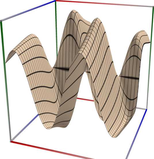
\[I_{\nu}\left(z\right) = z^{\nu} (iz)^{-\nu} J_{\nu}(iz) = \frac{1}{\Gamma(\nu+1)} \left(\frac{z}{2}\right)^{\nu} {}_0F_1\left(\nu+1, \frac{z^2}{4}\right).\]

The wpf figures below are showing the real part (left figure), imaginary part (middle figure) and absolute value with color-coded phase (right figure) of the complex function \(z = I_{\nu}(x + iy)\) with \(\nu=0\) and \(-6 \le x \le 6\) (blue axis), \(-6 \le y \le 6\) (red axis), \(-10 \le z \le 10\) (green axis). Function values are loglog-transformed.

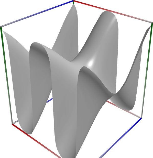\(\quad\) 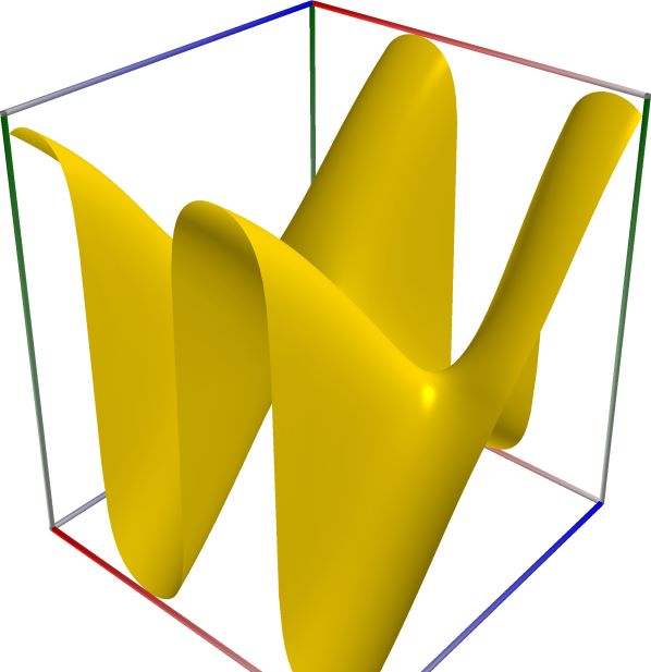\(\quad\)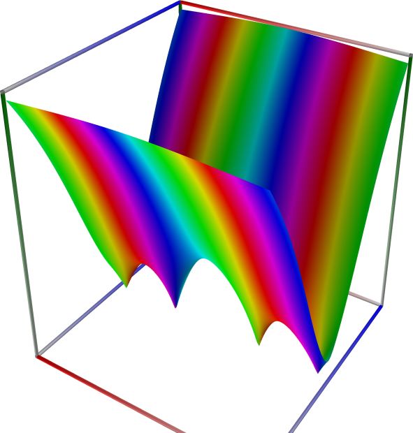

The corresponding scaled function looks like this:

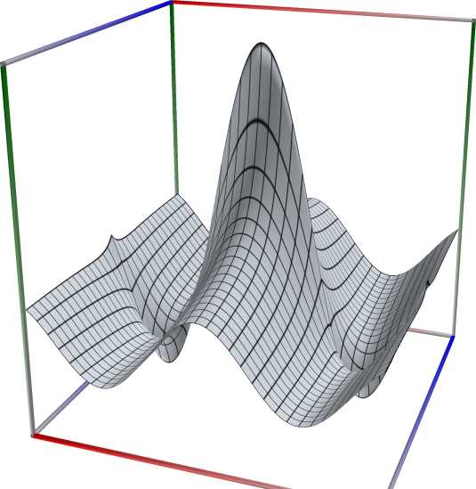\(\quad\) \(\quad\)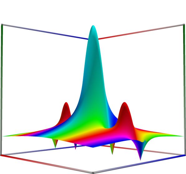

An example in Python

>>> from xlcalcnet import xreal
>>> xreal.BesselI(3, 0.5)
xreal('5.2359877559829887307E-1')
>>> xreal.BesselI(3, '0.51')
xreal('5.3518479027559984754E-1')

An example in Visual Basic

>>> from xlcalcnet import Gpr
>>> Gpr.BesselI(3, 0.5)
Gpr('5.2359877559829887307E-1')
>>> Gpr.BesselI(3, '0.51')
Gpr('5.3518479027559984754E-1')

An example with real input:

>>> from xlcalcnet import dec, mpm, gmp, fpm, apm
>>> mpm.dps = 40; n= 10; x = 30
>>> \mathrm{d}x = dec.besseli(n, x); mx = mpm.besseli(n, x); gx = gmp.besseli(n, x)
>>> fx = fpm.besseli(n, x); ax = apm.besseli(n, x)
>>> mpm.show([\mathrm{d}x, mx, gx, fx, ax])
dec:  1.458318099759671237651634761704819246948E+11
mpm:  1.458318099759671237651634761704819246948e+11
gmp:  1.458318099759671237651634761704819246948E+11
fpm:  1.45831809975967E+11
apm:  1.458318099759671237651634761704819246948e+11 (2.164e-39%)

An example with complex input:

>>> from xlcalcnet import dec, mpm, gmp, fpm, apm
>>> mpm.dps = 20; n= 10; z = '3 + 4j'
>>> \mathrm{d}z = dec.besseli(n, z); mz = mpm.besseli(n, z); gz = gmp.besseli(n, z)
>>> fz = fpm.besseli(n, z); az = apm.besseli(n, z)
>>> mpm.show([\mathrm{d}z, mz, gz, fz, az],  aligned=True)
dec: -2.0890476012080940545E-3               - 8.8394935038889455024E-4j
mpm: -2.0890476012080940545e-3               - 8.8394935038889455024e-4j
gmp: -2.0890476012080940545E-03              - 8.8394935038889455024E-04j
fpm: -2.08904760120809E-03                   - 8.83949350388895E-04j
apm: -2.0890476012080940545e-3 (-7.919e-20%) - 8.8394935038889455024e-4 (-9.358e-20%)j

Modified Bessel function of the 2nd kind, \(K_{\nu}(x)\)

ctx.bessel_kv(x, nu, scaled=False)

Returns \(K_{\nu}(x)\), the modified Bessel function of the second kind.

If scaled is True, then \(K_{\nu}(x) \cdot \exp(x)\) is returned.

See also Wikipedia [1370], MathWorld [981], NIST [469], BoostMath [114], Ehrhardt [309] (3.1.4.3), Flint [822], Flint [820], Mpmath [625].

If ctx is math53, ctxboost or ctxflintreal, then \(\nu, x \in \mathbb{R}\) is exspected. If ctx is cmath53, then \(\nu \in \mathbb{R}\) and \(x \in \mathbb{C}\) is exspected. If ctx is ctxflintcplx then \(\nu, x \in \mathbb{C}\) is accepted.

The function is defined as

\[K_{\nu}\left(z\right)=\tfrac{1}{2}\pi\frac{I_{-\nu}\left(z\right)-I_{\nu}\left(z\right)}{\sin\left(\nu\pi\right)}.\]

if \(\nu \notin \mathbb{Z}\). If \(\nu \in \mathbb{Z}\), it computes the limit value.

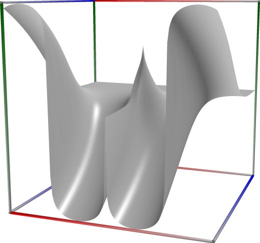
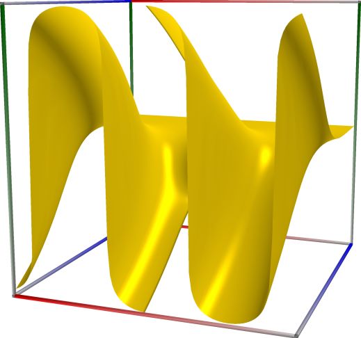
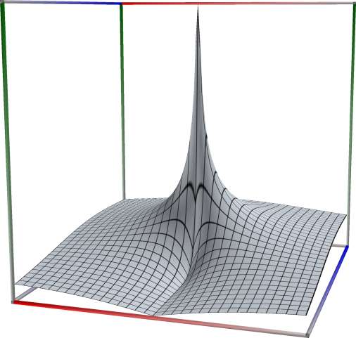
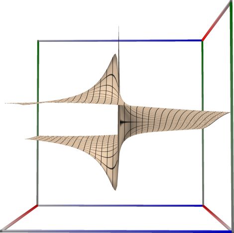
The wpf figures below are showing the real part (left figure), imaginary part (middle figure) and absolute value with color-coded phase (right figure) of the complex function \(z = K_{\nu}(x + iy)\) with \(\nu=0\) and \(-6 \le x \le 6\) (blue axis), \(-6 \le y \le 6\) (red axis), \(-10 \le z \le 10\) (green axis). Function values are loglog-transformed.

\(\quad\) \(\quad\)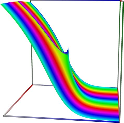

The corresponding scaled function looks like this:

\(\quad\) \(\quad\)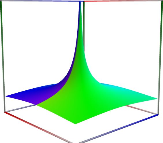

An example in Python

>>> from xlcalcnet import xreal
>>> xreal.BesselK(3, 0.5)
xreal('5.2359877559829887307E-1')
>>> xreal.BesselK(3, '0.51')
xreal('5.3518479027559984754E-1')

An example in Visual Basic

>>> from xlcalcnet import Gpr
>>> Gpr.BesselK(3, 0.5)
Gpr('5.2359877559829887307E-1')
>>> Gpr.BesselK(3, '0.51')
Gpr('5.3518479027559984754E-1')

An example with real input:

>>> from xlcalcnet import dec, mpm, gmp, fpm, apm
>>> mpm.dps = 40; n= 10; x = 30
>>> \mathrm{d}x = dec.besselk(n, x); mx = mpm.besselk(n, x); gx = gmp.besselk(n, x)
>>> fx = fpm.besselk(n, x); ax = apm.besselk(n, x)
>>> mpm.show([\mathrm{d}x, mx, gx, fx, ax])
dec:  1.084281694222297391103753613581684920880E-13
mpm:  1.084281694222297391103753613581684920880e-13
gmp:  1.084281694222297391103753613581684920880E-13
fpm:  1.08428169422230E-13
apm:  1.084281694222297390843838224178185275164e-13 (1.245e-14%)

An example with complex input:

>>> from xlcalcnet import dec, mpm, gmp, fpm, apm
>>> mpm.dps = 20; n= 10; z = '3 + 4j'
>>> \mathrm{d}z = dec.besselk(n, z); mz = mpm.besselk(n, z); gz = gmp.besselk(n, z)
>>> fz = fpm.besselk(n, z); az = apm.besselk(n, z)
>>> mpm.show([\mathrm{d}z, mz, gz, fz, az],  aligned=True)
dec: -1.9416209202983682785E+1               + 1.1318334583389307477E+1j
mpm: -1.9416209202983682785e+1               + 1.1318334583389307477e+1j
gmp: -1.9416209202983682785E+01              + 1.1318334583389307477E+01j
fpm: -1.94162092029837E+01                   + 1.13183345833893E+01j
apm: -1.9416209202983682785e+1 (-2.792e-19%) + 1.1318334583389307477e+1 (3.592e-19%)j

First derivative of the modified Bessel function of the first kind \(I'_{\nu}(x)\)

ctx.bessel_iv_prime(x, nu, scaled=False)

Returns \(I'_{\nu}(x)\), the first derivative (with respect to \(x\)) of \(I_{\nu}(z)\), the modified Bessel function of the first kind

If scaled is True, then \(I'_{\nu}(x) \cdot \exp(-|\Re(x)|)\) is returned.

See also Wikipedia [1370], MathWorld [980], NIST [468], BoostMath [114], BoostMath [122].

If ctx is math53, ctxboost or ctxflintreal, then \(\nu, x \in \mathbb{R}\) is exspected. If ctx is cmath53, then \(\nu \in \mathbb{R}\) and \(x \in \mathbb{C}\) is exspected. If ctx is ctxflintcplx then \(\nu, x \in \mathbb{C}\) is accepted.

The function is calculated as \(I'_{\nu}(x) = \tfrac{1}{2} (I_{\nu-1}(x) + I_{\nu+1}(x))\).

An example in Python

>>> from xlcalcnet import xreal
>>> xreal.BesselIPrime(3, 0.5)
xreal('5.2359877559829887307E-1')
>>> xreal.BesselIPrime(3, '0.51')
xreal('5.3518479027559984754E-1')

An example in Visual Basic

>>> from xlcalcnet import Gpr
>>> Gpr.BesselIPrime(3, 0.5)
Gpr('5.2359877559829887307E-1')
>>> Gpr.BesselIPrime(3, '0.51')
Gpr('5.3518479027559984754E-1')

First derivative of the modified Bessel function of the second kind \(K'_{\nu}(x)\)

ctx.bessel_kv_prime(x, nu, scaled=False)

Returns \(K'_{\nu}(x)\), the first derivative (with respect to \(x\)) of \(K_{\nu}(x)\), the modified Bessel function of the second kind.

If scaled is True, then \(K'_{\nu}(x) \cdot \exp(x)\) is returned.

See also Wikipedia [1356], MathWorld [951], NIST [463], BoostMath [100], BoostMath [122].

If ctx is math53, ctxboost or ctxflintreal, then \(\nu, x \in \mathbb{R}\) is exspected. If ctx is cmath53, then \(\nu \in \mathbb{R}\) and \(x \in \mathbb{C}\) is exspected. If ctx is ctxflintcplx then \(\nu, x \in \mathbb{C}\) is accepted.

The function is calculated as \(K'_{\nu}(x) = -\tfrac{1}{2} (K_{\nu-1}(x) + K_{\nu+1}(x))\).

An example with real input:

>>> from xlcalcnet import dec, mpm, gmp, fpm, apm
>>> mpm.dps = 20; n= 10; x = 30
>>> \mathrm{d}x = dec.hankel1(n, x); mx = mpm.hankel1(n, x); gx = gmp.hankel1(n, x)
>>> fx = fpm.hankel1(n, x); ax = apm.hankel1(n, x)
>>> mpm.show([\mathrm{d}x, mx, gx, fx, ax],  aligned=True)
dec: -1.2987689399858876819E-1               + 7.5056702122397113289E-2j
mpm: -1.2987689399858876819e-1               + 7.5056702122397113289e-2j
gmp: -1.2987689399858876819E-01              + 7.5056702122397113289E-02j
fpm: -1.29876893998589E-01                   + 7.50567021223971E-02j
apm: -1.2987689399889094748e-1 (-9.932e-10%) + 7.5056702113900822249e-2 (2.838e-6%)j

An example with complex input:

>>> from xlcalcnet import dec, mpm, gmp, fpm, apm
>>> mpm.dps = 20; n= 10; z = '3 + 4j'
>>> \mathrm{d}z = dec.hankel1(n, z); mz = mpm.hankel1(n, z); gz = gmp.hankel1(n, z)
>>> fz = fpm.hankel1(n, z); az = apm.hankel1(n, z)
>>> mpm.show([\mathrm{d}z, mz, gz, fz, az],  aligned=True)
dec: -6.9984001073685610955E+0              + 6.7915518863025118064E+0j
mpm: -6.9984001073685610955e+0              + 6.7915518863025118064e+0j
gmp: -6.9984001073685610955E+00             + 6.7915518863025118064E+00j
fpm: -6.99840010736856E+00                  + 6.79155188630251E+00j
apm: -6.9984001073685610955e+0 (-2.13e-18%) + 6.7915518863025118064e+0 (2.145e-18%)j

Marcum Q function, \(Q_m(a,b)\) (up to octuple precision)

math53.marcum_q(m, a, b)

Returns the Marcum Q-function \(\displaystyle Q_m(a,b)= \frac{1}{a^{m-1}} \int _{b}^{\infty} x^m \exp \left(-{\frac {x^{2}+a^{2}}{2}}\right)I_{m-1}(ax) \, \mathrm{d}x\), where \(m>0\), \(b\geq 0\), \(a>0\) and \(I_{m-1}\) is the modified Bessel function of first kind of order \(m-1\).

See also: Short [525], Wikipedia [1459], MathWorld [1087], Ehrhardt [309] (3.3.17).

It is calculated using its relationship to the noncentral chi-squared cumulative distribution function:

If \(X\sim \chi _{k}^{2}(\lambda )\) is a non-central chi-squared distribution with non-centrality parameter \(\lambda\) and \(k\) degrees of freedom, then its cdf is given by \(\displaystyle F_{X}(x)=1-Q_{k/2}({\sqrt {\lambda }},{\sqrt {x}})\).

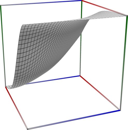
Left figure: real (“silver”) and imaginary (“gold”) part of the Marcum Q function, \(Q_m(a,b)\). Camera angles are \(\theta=135^\circ\) and \(\phi = -12^\circ\), camera radius is -2.

An example in Python

>>> from xlcalcnet import xreal
>>> xreal.MarcumQ(2, 3 ,0.5)
xreal('5.2359877559829887307E-1')
>>> xreal.MarcumQ(2.4, 3.6, ' 0.51')
xreal('5.3518479027559984754E-1')

An example in Visual Basic

>>> from xlcalcnet import Gpr
>>> Gpr.MarcumQ(2, 3 ,0.5)
Gpr('5.2359877559829887307E-1')
>>> Gpr.MarcumQ(2.4, 3.6, ' 0.51')
Gpr('5.3518479027559984754E-1')