Jacobi elliptic functions

For an introduction, see Wikipedia [1417], MathWorld [1038], BoostMath [159], NIST [501], Mpmath [687].

Jacobi elliptic function \(\mathrm{sn}(x, k)\)

ctx.jacobi_sn(x, k)

where ctx is math53, mathc53 or ctxboost.

Returns the Jacobi elliptic function \(\mathrm{sn}(x, k) = \sin(\mathrm{am}(x, k))\), where \(\mathrm{am}(x, k)\) denotes the Jacobi amplitude function, and \(\mathrm{sn}(x, 0) = \sin(x)\). See also BoostMath [164], Wikipedia [1417], MathWorld [285], NIST [501], Ehrhardt [309] (3.2.11.1), Ehrhardt [309] (4.2.58).

The version for XComplex has the restriction that \(k\) must be real.

\(\quad\) \(\quad\)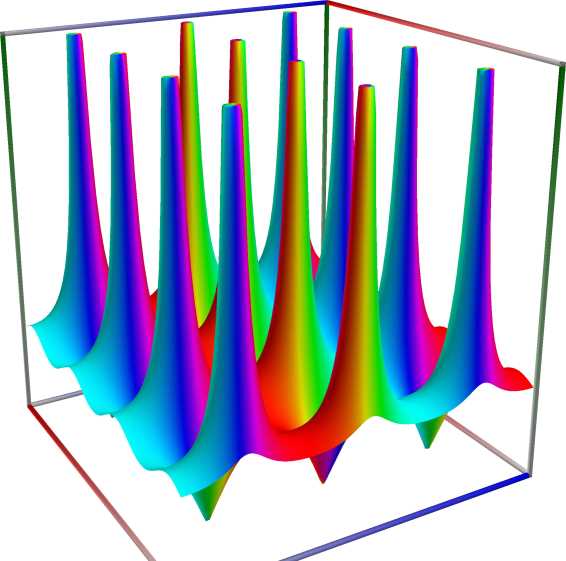

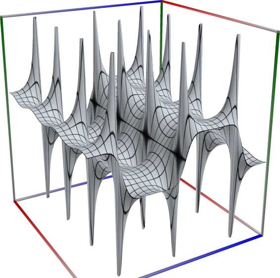
Left figure: real part of the Jacobi elliptic function sn(\(z, k\)). Camera angles are \(\theta=135^\circ\) and \(\phi = -12^\circ\), camera radius is -2.

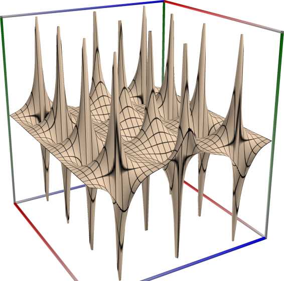
Middle figure: imaginary part of the Jacobi elliptic function sn(\(z, k\)). Camera angles are \(\theta=135^\circ\) and \(\phi = -12^\circ\), camera radius is -2.

Right figure: absolute value of the Jacobi elliptic function sn(\(z, k\)), with color-coded phase. Camera angles are \(\theta=135^\circ\) and \(\phi = -12^\circ\), camera radius is -2.

An example in Python

>>> from xlcalcnet import xreal
>>> xreal.JacobiSN(0.8, 0.5)
xreal('5.2359877559829887307E-1')
>>> xreal.JacobiSN(0.8, '0.51')
xreal('5.3518479027559984754E-1')

An example in Visual Basic

>>> from xlcalcnet import Gpr
>>> Gpr.JacobiSN(0.8, 0.5)
Gpr('5.2359877559829887307E-1')
>>> Gpr.JacobiSN(0.8, '0.51')
Gpr('5.3518479027559984754E-1')

The function is defined as

\[\mathrm{sn}(u,k) = \frac{\theta_3(0,q)}{\theta_2(0,q)} \frac{\theta_1(t,q)}{\theta_4(t,q)}.\]

Here \(t = u/\theta^2_3(0,q)\), \(q = q(k) = \exp \left[ -\pi K'(k) / K(k) \right]\) denotes the nome, \(K(k)\) denotes the complete elliptic integral of the first kind and \(K'(k) = K(\sqrt{1-k^2})\) denotes the complementary complete elliptic integral of the first kind.

An example with real input:

>>> from xlcalcnet import dec, mpm, gmp, fpm, apm
>>> mpm.dps = 40; u = '11.0'; m = '0.6'
>>> \mathrm{d}x = dec.jacobi_sn(u, m); mx = mpm.jacobi_sn(u, m); gx = gmp.jacobi_sn(u, m)
>>> fx = fpm.jacobi_sn(u, m); ax = apm.jacobi_sn(u, m)
>>> mpm.show([\mathrm{d}x, mx, gx, fx, ax])
dec:  6.185656260215812572753605488481047900065E-1
mpm:  6.185656260215812572753605488481047900065e-1
gmp:  6.185656260215812572753605488481047900065E-01
fpm:  6.18565626021581E-01
apm:  6.185656260215812572753605488481047900065e-1 (9.279e-40%)

An example with complex input:

>>> from xlcalcnet import dec, mpm, gmp, fpm, apm
>>> mpm.dps = 20; u = '11.0 + 2.0j'; m = '0.6'
>>> \mathrm{d}z = dec.jacobi_sn(u, m); mz = mpm.jacobi_sn(u, m); gz = gmp.jacobi_sn(u, m)
>>> fz = fpm.jacobi_sn(u, m); az = apm.jacobi_sn(u, m)
>>> mpm.show([\mathrm{d}z, mz, gz, fz, az], aligned=True)
dec: 1.9171467233805943128E+0              + 4.6311952375545897275E-1j
mpm: 1.9171467233805943128e+0              + 4.6311952375545897275e-1j
gmp: 1.9171467233805943128E+00             + 4.6311952375545897275E-01j
fpm: 1.91714672338059E+00                  + 4.63119523755459E-01j
apm: 1.9171467233805943128e+0 (4.418e-20%) + 4.6311952375545897275e-1 (4.572e-20%)j

Jacobi elliptic function \(\mathrm{cn}(x, k)\)

ctx.jacobi_cn(x, k)

where ctx is math53, mathc53 or ctxboost.

Returns the Jacobi elliptic function \(\mathrm{cn}(x, k) = \cos(\mathrm{am}(x, k))\), where \(\mathrm{am}(x, k)\) denotes the Jacobi amplitude function, and \(\mathrm{cn}(x, 0) = \cos(x)\). See also BoostMath [149], Wikipedia [1417], MathWorld [275], NIST [501], Ehrhardt [309] (3.2.11.2), Ehrhardt [309] (4.2.18).

The version for XComplex has the restriction that \(k\) must be real.

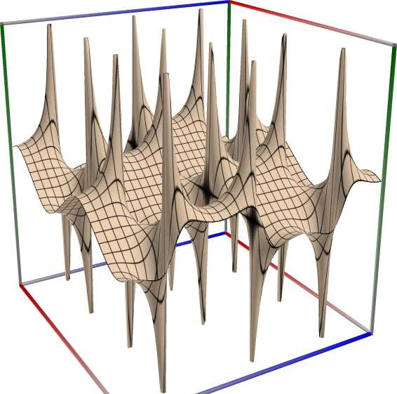
\(\quad\) \(\quad\)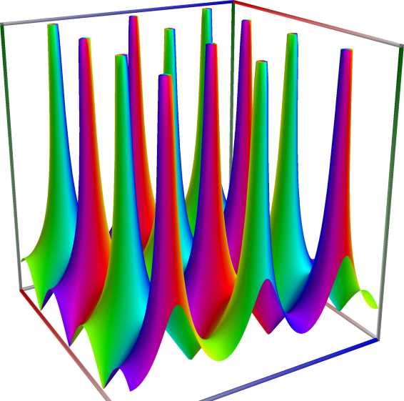

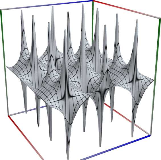
Left figure: real part of the Jacobi elliptic function cn(\(z, k\)). Camera angles are \(\theta=135^\circ\) and \(\phi = -12^\circ\), camera radius is -2.

Middle figure: imaginary part of the Jacobi elliptic function cn(\(z, k\)). Camera angles are \(\theta=135^\circ\) and \(\phi = -12^\circ\), camera radius is -2.

Right figure: absolute value of the Jacobi elliptic function cn(\(z, k\)), with color-coded phase. Camera angles are \(\theta=135^\circ\) and \(\phi = -12^\circ\), camera radius is -2.

An example in Python

>>> from xlcalcnet import xreal
>>> xreal.JacobiCN(0.8, 0.5)
xreal('5.2359877559829887307E-1')
>>> xreal.JacobiCN(0.8, '0.51')
xreal('5.3518479027559984754E-1')

An example in Visual Basic

>>> from xlcalcnet import Gpr
>>> Gpr.JacobiCN(0.8, 0.5)
Gpr('5.2359877559829887307E-1')
>>> Gpr.JacobiCN(0.8, '0.51')
Gpr('5.3518479027559984754E-1')

The function is defined as

\[\mathrm{cn}(u,k) = \frac{\theta_4(0,q)}{\theta_2(0,q)} \frac{\theta_2(t,q)}{\theta_4(t,q)}.\]

Here \(t = u/\theta^2_3(0,q)\), and \(q = q(k)\) denotes the nome.

An example with real input:

>>> from xlcalcnet import dec, mpm, gmp, fpm, apm
>>> mpm.dps = 40; u = '11.0'; m = '0.6'
>>> \mathrm{d}x = dec.jacobi_cn(u, m); mx = mpm.jacobi_cn(u, m); gx = gmp.jacobi_cn(u, m)
>>> fx = fpm.jacobi_cn(u, m); ax = apm.jacobi_cn(u, m)
>>> mpm.show([\mathrm{d}x, mx, gx, fx, ax])
dec:  -7.857331393701867250820479479353994215372E-1
mpm:  -7.857331393701867250820479479353994215372e-1
gmp:  -7.857331393701867250820479479353994215372E-01
fpm:  -7.85733139370187E-01
apm:  -7.857331393701867250820479479353994215373e-1 (-7.305e-40%)

An example with complex input:

>>> from xlcalcnet import dec, mpm, gmp, fpm, apm
>>> mpm.dps = 20; u = '11.0 + 2.0j'; m = '0.6'
>>> \mathrm{d}z = dec.jacobi_cn(u, m); mz = mpm.jacobi_cn(u, m); gz = gmp.jacobi_cn(u, m)
>>> fz = fpm.jacobi_cn(u, m); az = apm.jacobi_cn(u, m)
>>> mpm.show([\mathrm{d}z, mz, gz, fz, az], aligned=True)
dec: 5.3561363916431377722E-1              - 1.6576651761270445419E+0j
mpm: 5.3561363916431377722e-1              - 1.6576651761270445419e+0j
gmp: 5.3561363916431377722E-01             - 1.6576651761270445419E+00j
fpm: 5.35613639164314E-01                  - 1.65766517612704E+00j
apm: 5.3561363916431377721e-1 (7.907e-20%) - 1.6576651761270445419e+0 (-5.11e-20%)j

Jacobi elliptic function \(\mathrm{dn}(x, k)\)

ctx.jacobi_dn(x, k)

where ctx is math53, mathc53 or ctxboost.

Returns the Jacobi elliptic function \(\mathrm{dn}(x, k) = \sqrt{1 - k^2 \mathrm{sn}^2(x, k)}\) with \(\mathrm{dn}(x, 0) = 1\). See also BoostMath [152], Wikipedia [1417], MathWorld [278], NIST [501], Ehrhardt [309] (3.2.11.3), Ehrhardt [309] (4.2.26).

The version for XComplex has the restriction that \(k\) must be real.

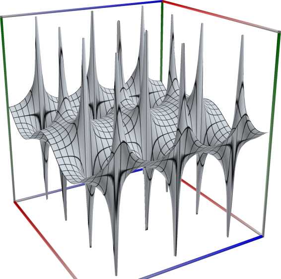\(\quad\) 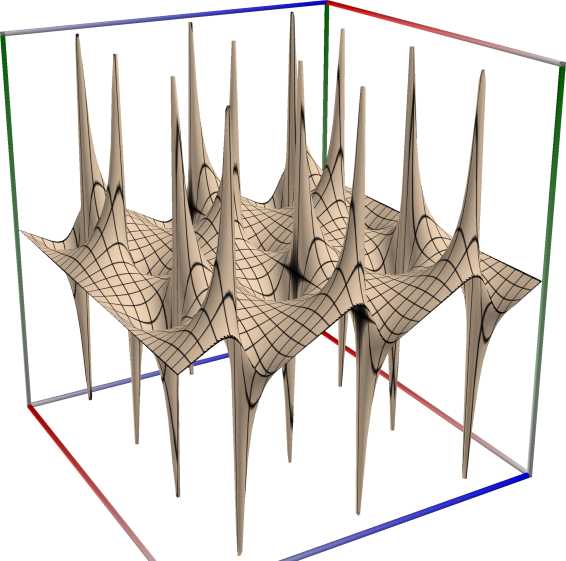\(\quad\)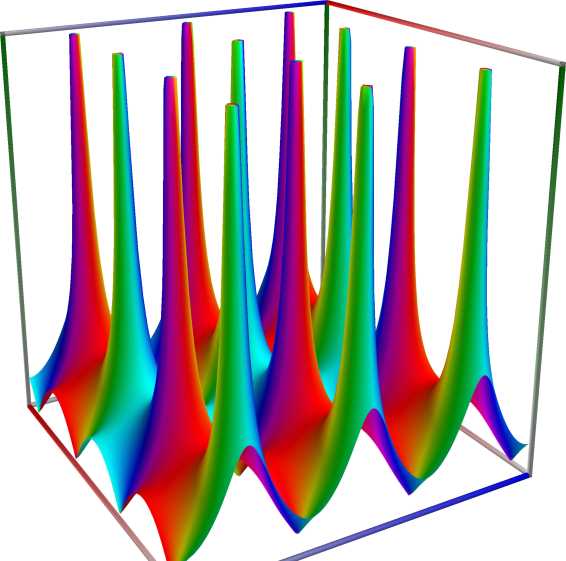

Left figure: real part of the Jacobi elliptic functions dn(\(z, k\)). Camera angles are \(\theta=135^\circ\) and \(\phi = -12^\circ\), camera radius is -2.

Middle figure: imaginary part of the Jacobi elliptic functions dn(\(z, k\)). Camera angles are \(\theta=135^\circ\) and \(\phi = -12^\circ\), camera radius is -2.

Right figure: absolute value of the Jacobi elliptic functions dn(\(z, k\)), with color-coded phase. Camera angles are \(\theta=135^\circ\) and \(\phi = -12^\circ\), camera radius is -2.

An example in Python

>>> from xlcalcnet import xreal
>>> xreal.JacobiDN(0.8, 0.5)
xreal('5.2359877559829887307E-1')
>>> xreal.JacobiDN(0.8, '0.51')
xreal('5.3518479027559984754E-1')

An example in Visual Basic

>>> from xlcalcnet import Gpr
>>> Gpr.JacobiDN(0.8, 0.5)
Gpr('5.2359877559829887307E-1')
>>> Gpr.JacobiDN(0.8, '0.51')
Gpr('5.3518479027559984754E-1')

The function is defined as

\[\mathrm{dn}(u,k) = \frac{\theta_4(0,q)}{\theta_3(0,q)} \frac{\theta_3(t,q)}{\theta_4(t,q)}.\]

Here \(t = u/\theta^2_3(0,q)\), and \(q = q(k)\) denotes the nome.

An example with real input:

>>> from xlcalcnet import dec, mpm, gmp, fpm, apm
>>> mpm.dps = 40; u = '11.0'; m = '0.6'
>>> \mathrm{d}x = dec.jacobi_dn(u, m); mx = mpm.jacobi_dn(u, m); gx = gmp.jacobi_dn(u, m)
>>> fx = fpm.jacobi_dn(u, m); ax = apm.jacobi_dn(u, m)
>>> mpm.show([\mathrm{d}x, mx, gx, fx, ax])
dec:  8.777391069006311317801212171013768906043E-1
mpm:  8.777391069006311317801212171013768906043e-1
gmp:  8.777391069006311317801212171013768906043E-01
fpm:  8.77739106900631E-01
apm:  8.777391069006311317801212171013768906043e-1 (6.539e-40%)

An example with complex input:

>>> from xlcalcnet import dec, mpm, gmp, fpm, apm
>>> mpm.dps = 20; u = '11.0 + 2.0j'; m = '0.6'
>>> \mathrm{d}z = dec.jacobi_dn(u, m); mz = mpm.jacobi_dn(u, m); gz = gmp.jacobi_dn(u, m)
>>> fz = fpm.jacobi_dn(u, m); az = apm.jacobi_dn(u, m)
>>> mpm.show([\mathrm{d}z, mz, gz, fz, az], aligned=True)
dec: -4.6801583272820746144E-1               + 1.1382538992226457533E+0j
mpm: -4.6801583272820746144e-1               + 1.1382538992226457533e+0j
gmp: -4.6801583272820746144E-01              + 1.1382538992226457533E+00j
fpm: -4.68015832728208E-01                   + 1.13825389922265E+00j
apm: -4.6801583272820746143e-1 (-4.525e-20%) + 1.1382538992226457533e+0 (7.442e-20%)j

Jacobi elliptic function \(\mathrm{nc}(x, k)\)

ctx.jacobi_nc(x, k)

where ctx is math53 or ctxboost.

Returns the Jacobi elliptic function \(\mathrm{nc}(x, k) = 1/\mathrm{cn}(x, k)\), with \(\mathrm{nc}(x, 0) = 1/\cos(x)\). See also BoostMath [154], Wikipedia [1417], MathWorld [280], NIST [501], Ehrhardt [309] (3.2.11.4).

An example in Python

>>> from xlcalcnet import xreal
>>> xreal.JacobiNC(0.8, 0.5)
xreal('5.2359877559829887307E-1')
>>> xreal.JacobiNC(0.8, '0.51')
xreal('5.3518479027559984754E-1')

An example in Visual Basic

>>> from xlcalcnet import Gpr
>>> Gpr.JacobiNC(0.8, 0.5)
Gpr('5.2359877559829887307E-1')
>>> Gpr.JacobiNC(0.8, '0.51')
Gpr('5.3518479027559984754E-1')

The function is defined as

\[\mathrm{nc}(u,k) = \frac{1}{\mathrm{cn}(u,k)}.\]

An example with real input:

>>> from xlcalcnet import dec, mpm, gmp, fpm, apm
>>> mpm.dps = 40; u = '11.0'; m = '0.6'
>>> \mathrm{d}x = dec.jacobi_nc(u, m); mx = mpm.jacobi_nc(u, m); gx = gmp.jacobi_nc(u, m)
>>> fx = fpm.jacobi_nc(u, m); ax = apm.jacobi_nc(u, m)
>>> mpm.show([\mathrm{d}x, mx, gx, fx, ax])
dec:  -1.272696733653822082392877366275776826356E+0
mpm:  -1.272696733653822082392877366275776826356e+0
gmp:  -1.272696733653822082392877366275776826356E+00
fpm:  -1.27269673365382E+00
apm:  -1.272696733653822082392877366275776826356e+0 (-9.02e-40%)

An example with complex input:

>>> from xlcalcnet import dec, mpm, gmp, fpm, apm
>>> mpm.dps = 20; u = '11.0 + 2.0j'; m = '0.6'
>>> \mathrm{d}z = dec.jacobi_nc(u, m); mz = mpm.jacobi_nc(u, m); gz = gmp.jacobi_nc(u, m)
>>> fz = fpm.jacobi_nc(u, m); az = apm.jacobi_nc(u, m)
>>> mpm.show([\mathrm{d}z, mz, gz, fz, az], aligned=True)
dec: 1.7649432217423873247E-1              + 5.4623047334802764261E-1j
mpm: 1.7649432217423873247e-1              + 5.4623047334802764261e-1j
gmp: 1.7649432217423873247E-01             + 5.4623047334802764261E-01j
fpm: 1.76494322174239E-01                  + 5.46230473348028E-01j
apm: 1.7649432217423873247e-1 (5.999e-20%) + 5.4623047334802764261e-1 (7.753e-20%)j

Jacobi elliptic function \(\mathrm{sc}(x, k)\)

ctx.jacobi_sc(x, k)

where ctx is math53 or ctxboost.

Returns the Jacobi elliptic function \(\mathrm{sc}(x, k) = \mathrm{sn}(x, k)/\mathrm{cn}(x, k)\). See also BoostMath [157], Wikipedia [1417], MathWorld [283], NIST [501], Ehrhardt [309] (3.2.11.5).

An example in Python

>>> from xlcalcnet import xreal
>>> xreal.JacobiSC(0.8, 0.5)
xreal('5.2359877559829887307E-1')
>>> xreal.JacobiSC(0.8, '0.51')
xreal('5.3518479027559984754E-1')

An example in Visual Basic

>>> from xlcalcnet import Gpr
>>> Gpr.JacobiSC(0.8, 0.5)
Gpr('5.2359877559829887307E-1')
>>> Gpr.JacobiSC(0.8, '0.51')
Gpr('5.3518479027559984754E-1')

The function is defined as

\[\mathrm{sc}(u,k) = \frac{\mathrm{sn}(u,k)}{\mathrm{cn}(u,k)}.\]

An example with real input:

>>> from xlcalcnet import dec, mpm, gmp, fpm, apm
>>> mpm.dps = 40; u = '11.0'; m = '0.6'
>>> \mathrm{d}x = dec.jacobi_sc(u, m); mx = mpm.jacobi_sc(u, m); gx = gmp.jacobi_sc(u, m)
>>> fx = fpm.jacobi_sc(u, m); ax = apm.jacobi_sc(u, m)
>>> mpm.show([\mathrm{d}x, mx, gx, fx, ax])
dec:  -7.872464517881981193304679205001097295818E-1
mpm:  -7.872464517881981193304679205001097295818e-1
gmp:  -7.872464517881981193304679205001097295818E-01
fpm:  -7.87246451788198E-01
apm:  -7.872464517881981193304679205001097295818e-1 (-7.291e-40%)

An example with complex input:

>>> from xlcalcnet import dec, mpm, gmp, fpm, apm
>>> mpm.dps = 20; u = '11.0 + 2.0j'; m = '0.6'
>>> \mathrm{d}z = dec.jacobi_sc(u, m); mz = mpm.jacobi_sc(u, m); gz = gmp.jacobi_sc(u, m)
>>> fz = fpm.jacobi_sc(u, m); az = apm.jacobi_sc(u, m)
>>> mpm.show([\mathrm{d}z, mz, gz, fz, az], aligned=True)
dec: 8.5395514773963269121E-2              + 1.1289419286206782292E+0j
mpm: 8.5395514773963269121e-2              + 1.1289419286206782292e+0j
gmp: 8.5395514773963269121E-02             + 1.1289419286206782292E+00j
fpm: 8.53955147739632E-02                  + 1.12894192862068E+00j
apm: 8.5395514773963269121e-2 (6.199e-20%) + 1.1289419286206782292e+0 (7.503e-20%)j

Jacobi elliptic function \(\mathrm{dc}(x, k)\)

ctx.jacobi_dc(x, k)

where ctx is math53 or ctxboost.

Returns the Jacobi elliptic function \(\mathrm{dc}(x, k) = \mathrm{dn}(x, k)/\mathrm{cn}(x, k)\). See also BoostMath [151], Wikipedia [1417], MathWorld [277], NIST [501], Ehrhardt [309] (3.2.11.6).

An example in Python

>>> from xlcalcnet import xreal
>>> xreal.JacobiDC(0.8, 0.5)
xreal('5.2359877559829887307E-1')
>>> xreal.JacobiDC(0.8, '0.51')
xreal('5.3518479027559984754E-1')

An example in Visual Basic

>>> from xlcalcnet import Gpr
>>> Gpr.JacobiDC(0.8, 0.5)
Gpr('5.2359877559829887307E-1')
>>> Gpr.JacobiDC(0.8, '0.51')
Gpr('5.3518479027559984754E-1')

The function is defined as

\[\mathrm{dc}(u,k) = \frac{\mathrm{dn}(u,k)}{\mathrm{cn}(u,k)}.\]

An example with real input:

>>> from xlcalcnet import dec, mpm, gmp, fpm, apm
>>> mpm.dps = 40; u = '11.0'; m = '0.6'
>>> \mathrm{d}x = dec.jacobi_dc(u, m); mx = mpm.jacobi_dc(u, m); gx = gmp.jacobi_dc(u, m)
>>> fx = fpm.jacobi_dc(u, m); ax = apm.jacobi_dc(u, m)
>>> mpm.show([\mathrm{d}x, mx, gx, fx, ax])
dec:  -1.117095694352656207726087789639773806912E+0
mpm:  -1.117095694352656207726087789639773806912e+0
gmp:  -1.117095694352656207726087789639773806912E+00
fpm:  -1.11709569435266E+00
apm:  -1.117095694352656207726087789639773806912e+0 (-1.028e-39%)

An example with complex input:

>>> from xlcalcnet import dec, mpm, gmp, fpm, apm
>>> mpm.dps = 20; u = '11.0 + 2.0j'; m = '0.6'
>>> \mathrm{d}z = dec.jacobi_dc(u, m); mz = mpm.jacobi_dc(u, m); gz = gmp.jacobi_dc(u, m)
>>> fz = fpm.jacobi_dc(u, m); az = apm.jacobi_dc(u, m)
>>> mpm.show([\mathrm{d}z, mz, gz, fz, az], aligned=True)
dec: -7.0435110332680081506E-1               - 5.4749159440014983159E-2j
mpm: -7.0435110332680081506e-1               - 5.4749159440014983159e-2j
gmp: -7.0435110332680081506E-01              - 5.4749159440014983159E-02j
fpm: -7.04351103326801E-01                   - 5.47491594400150E-02j
apm: -7.0435110332680081505e-1 (-6.013e-20%) - 5.4749159440014983159e-2 (-4.835e-20%)j

Jacobi elliptic function \(\mathrm{nd}(x, k)\)

ctx.jacobi_nd(x, k)

where ctx is math53 or ctxboost.

Returns the Jacobi elliptic function \(\mathrm{nd}(x, k) = 1/\mathrm{dn}(x, k)\). See also BoostMath [155], Wikipedia [1417], MathWorld [281], NIST [501], Ehrhardt [309] (3.2.11.7).

An example in Python

>>> from xlcalcnet import xreal
>>> xreal.JacobiNC(0.8, 0.5)
xreal('5.2359877559829887307E-1')
>>> xreal.JacobiNC(0.8, '0.51')
xreal('5.3518479027559984754E-1')

An example in Visual Basic

>>> from xlcalcnet import Gpr
>>> Gpr.JacobiNC(0.8, 0.5)
Gpr('5.2359877559829887307E-1')
>>> Gpr.JacobiNC(0.8, '0.51')
Gpr('5.3518479027559984754E-1')

The function is defined as

\[\mathrm{nd}(u,k) = \frac{1}{\mathrm{dn}(u,k)}.\]

An example with real input:

>>> from xlcalcnet import dec, mpm, gmp, fpm, apm
>>> mpm.dps = 40; u = '11.0'; m = '0.6'
>>> \mathrm{d}x = dec.jacobi_nd(u, m); mx = mpm.jacobi_nd(u, m); gx = gmp.jacobi_nd(u, m)
>>> fx = fpm.jacobi_nd(u, m); ax = apm.jacobi_nd(u, m)
>>> mpm.show([\mathrm{d}x, mx, gx, fx, ax])
dec:  1.139290698270334703522055295154469970359E+0
mpm:  1.139290698270334703522055295154469970359e+0
gmp:  1.139290698270334703522055295154469970359E+00
fpm:  1.13929069827033E+00
apm:  1.139290698270334703522055295154469970359e+0 (1.008e-39%)

An example with complex input:

>>> from xlcalcnet import dec, mpm, gmp, fpm, apm
>>> mpm.dps = 20; u = '11.0 + 2.0j'; m = '0.6'
>>> \mathrm{d}z = dec.jacobi_nd(u, m); mz = mpm.jacobi_nd(u, m); gz = gmp.jacobi_nd(u, m)
>>> fz = fpm.jacobi_nd(u, m); az = apm.jacobi_nd(u, m)
>>> mpm.show([\mathrm{d}z, mz, gz, fz, az], aligned=True)
dec: -3.0899053138818164120E-1               - 7.5149098081843035989E-1j
mpm: -3.0899053138818164120e-1               - 7.5149098081843035989e-1j
gmp: -3.0899053138818164120E-01              - 7.5149098081843035989E-01j
fpm: -3.08990531388182E-01                   - 7.51490980818430E-01j
apm: -3.0899053138818164120e-1 (-6.853e-20%) - 7.5149098081843035989e-1 (-5.636e-20%)j

Jacobi elliptic function \(\mathrm{sd}(x, k)\)

ctx.jacobi_sd(x, k)

where ctx is math53 or ctxboost.

Returns the Jacobi elliptic function \(\mathrm{sd}(x, k) = \mathrm{sn}(x, k)/\mathrm{dn}(x, k)\). See also BoostMath [163], Wikipedia [1417], MathWorld [284], NIST [501], Ehrhardt [309] (3.2.11.8).

An example in Python

>>> from xlcalcnet import xreal
>>> xreal.JacobiSD(0.8, 0.5)
xreal('5.2359877559829887307E-1')
>>> xreal.JacobiSD(0.8, '0.51')
xreal('5.3518479027559984754E-1')

An example in Visual Basic

>>> from xlcalcnet import Gpr
>>> Gpr.JacobiSD(0.8, 0.5)
Gpr('5.2359877559829887307E-1')
>>> Gpr.JacobiSD(0.8, '0.51')
Gpr('5.3518479027559984754E-1')

The function is defined as

\[\mathrm{sd}(u,k) = \frac{\mathrm{sn}(u,k)}{\mathrm{dn}(u,k)}.\]

An example with real input:

>>> from xlcalcnet import dec, mpm, gmp, fpm, apm
>>> mpm.dps = 40; u = '11.0'; m = '0.6'
>>> \mathrm{d}x = dec.jacobi_sd(u, m); mx = mpm.jacobi_sd(u, m); gx = gmp.jacobi_sd(u, m)
>>> fx = fpm.jacobi_sd(u, m); ax = apm.jacobi_sd(u, m)
>>> mpm.show([\mathrm{d}x, mx, gx, fx, ax])
dec:  7.047260639961540287844417991398276789242E-1
mpm:  7.047260639961540287844417991398276789242e-1
gmp:  7.047260639961540287844417991398276789242E-01
fpm:  7.04726063996154E-01
apm:  7.047260639961540287844417991398276789242e-1 (8.145e-40%)

An example with complex input:

>>> from xlcalcnet import dec, mpm, gmp, fpm, apm
>>> mpm.dps = 20; u = '11.0 + 2.0j'; m = '0.6'
>>> \mathrm{d}z = dec.jacobi_sd(u, m); mz = mpm.jacobi_sd(u, m); gz = gmp.jacobi_sd(u, m)
>>> fz = fpm.jacobi_sd(u, m); az = apm.jacobi_sd(u, m)
>>> mpm.show([\mathrm{d}z, mz, gz, fz, az], aligned=True)
dec: -2.4435003966332689103E-1               - 1.5838180192675636948E+0j
mpm: -2.4435003966332689103e-1               - 1.5838180192675636948e+0j
gmp: -2.4435003966332689103E-01              - 1.5838180192675636948E+00j
fpm: -2.44350039663327E-01                   - 1.58381801926756E+00j
apm: -2.4435003966332689103e-1 (-4.333e-20%) - 1.5838180192675636948e+0 (-5.348e-20%)j

Jacobi elliptic function \(\mathrm{cd}(x, k)\)

ctx.jacobi_cd(x, k)

where ctx is math53 or ctxboost.

Returns the Jacobi elliptic function \(\mathrm{cd}(x, k) = \mathrm{cn}(x, k)/\mathrm{dn}(x, k)\). See also BoostMath [148], Wikipedia [1417], MathWorld [274], NIST [501], Ehrhardt [309] (3.2.11.9).

An example in Python

>>> from xlcalcnet import xreal
>>> xreal.JacobiCD(0.8, 0.5)
xreal('5.2359877559829887307E-1')
>>> xreal.JacobiCD(0.8, '0.51')
xreal('5.3518479027559984754E-1')

An example in Visual Basic

>>> from xlcalcnet import Gpr
>>> Gpr.JacobiCD(0.8, 0.5)
Gpr('5.2359877559829887307E-1')
>>> Gpr.JacobiCD(0.8, '0.51')
Gpr('5.3518479027559984754E-1')

The function is defined as

\[\mathrm{cd}(u,k) = \frac{\mathrm{cn}(u,k)}{\mathrm{dn}(u,k)}.\]

An example with real input:

>>> from xlcalcnet import dec, mpm, gmp, fpm, apm
>>> mpm.dps = 40; u = '11.0'; m = '0.6'
>>> \mathrm{d}x = dec.jacobi_cd(u, m); mx = mpm.jacobi_cd(u, m); gx = gmp.jacobi_cd(u, m)
>>> fx = fpm.jacobi_cd(u, m); ax = apm.jacobi_cd(u, m)
>>> mpm.show([\mathrm{d}x, mx, gx, fx, ax])
dec:  -8.951784570072022496881536952389380682250E-1
mpm:  -8.951784570072022496881536952389380682250e-1
gmp:  -8.951784570072022496881536952389380682250E-01
fpm:  -8.95178457007202E-01
apm:  -8.951784570072022496881536952389380682250e-1 (-6.412e-40%)

An example with complex input:

>>> from xlcalcnet import dec, mpm, gmp, fpm, apm
>>> mpm.dps = 20; u = '11.0 + 2.0j'; m = '0.6'
>>> \mathrm{d}z = dec.jacobi_cd(u, m); mz = mpm.jacobi_cd(u, m); gz = gmp.jacobi_cd(u, m)
>>> fz = fpm.jacobi_cd(u, m); az = apm.jacobi_cd(u, m)
>>> mpm.show([\mathrm{d}z, mz, gz, fz, az], aligned=True)
dec: -1.4112199720604079057E+0               + 1.0969402459986020016E-1j
mpm: -1.4112199720604079057e+0               + 1.0969402459986020016e-1j
gmp: -1.4112199720604079057E+00              + 1.0969402459986020016E-01j
fpm: -1.41121997206041E+00                   + 1.09694024599860E-01j
apm: -1.4112199720604079057e+0 (-6.002e-20%) + 1.0969402459986020016e-1 (4.826e-20%)j

Jacobi elliptic function \(\mathrm{ns}(x, k)\)

ctx.jacobi_ns(x, k)

where ctx is math53 or ctxboost.

Returns the Jacobi elliptic function \(\mathrm{ns}(x, k) =1/\mathrm{dn}(x, k)\). See also BoostMath [156], Wikipedia [1417], MathWorld [282], NIST [501], Ehrhardt [309] (3.2.11.10).

An example in Python

>>> from xlcalcnet import xreal
>>> xreal.JacobiNS(0.8, 0.5)
xreal('5.2359877559829887307E-1')
>>> xreal.JacobiNS(0.8, '0.51')
xreal('5.3518479027559984754E-1')

An example in Visual Basic

>>> from xlcalcnet import Gpr
>>> Gpr.JacobiNS(0.8, 0.5)
Gpr('5.2359877559829887307E-1')
>>> Gpr.JacobiNS(0.8, '0.51')
Gpr('5.3518479027559984754E-1')

The function is defined as

\[\mathrm{ns}(u,k) = \frac{1}{\mathrm{sn}(u,k)}.\]

An example with real input:

>>> from xlcalcnet import dec, mpm, gmp, fpm, apm
>>> mpm.dps = 40; u = '11.0'; m = '0.6'
>>> \mathrm{d}x = dec.jacobi_ns(u, m); mx = mpm.jacobi_ns(u, m); gx = gmp.jacobi_ns(u, m)
>>> fx = fpm.jacobi_ns(u, m); ax = apm.jacobi_ns(u, m)
>>> mpm.show([\mathrm{d}x, mx, gx, fx, ax])
dec:  1.616643340548494694635884305486544088759E+0
mpm:  1.616643340548494694635884305486544088759e+0
gmp:  1.616643340548494694635884305486544088759E+00
fpm:  1.61664334054850E+00
apm:  1.616643340548494694635884305486544088759e+0 (7.101e-40%)

An example with complex input:

>>> from xlcalcnet import dec, mpm, gmp, fpm, apm
>>> mpm.dps = 20; u = '11.0 + 2.0j'; m = '0.6'
>>> \mathrm{d}z = dec.jacobi_ns(u, m); mz = mpm.jacobi_ns(u, m); gz = gmp.jacobi_ns(u, m)
>>> fz = fpm.jacobi_ns(u, m); az = apm.jacobi_ns(u, m)
>>> mpm.show([\mathrm{d}z, mz, gz, fz, az], aligned=True)
dec: 4.9284848473105701998E-1              - 1.1905596621721617534E-1j
mpm: 4.9284848473105701998e-1              - 1.1905596621721617534e-1j
gmp: 4.9284848473105701998E-01             - 1.1905596621721617534E-01j
fpm: 4.92848484731057E-01                  - 1.19055966217216E-01j
apm: 4.9284848473105701998e-1 (4.297e-20%) - 1.1905596621721617534e-1 (-4.447e-20%)j

Jacobi elliptic function \(\mathrm{cs}(x, k)\)

ctx.jacobi_cs(x, k)

where ctx is math53 or ctxboost.

Returns the Jacobi elliptic function \(\mathrm{cs}(x, k) = \mathrm{cn}(x, k)/\mathrm{sn}(x, k)\). See also BoostMath [150], Wikipedia [1417], MathWorld [276], NIST [501], Ehrhardt [309] (3.2.11.11).

An example in Python

>>> from xlcalcnet import xreal
>>> xreal.JacobiCS(0.8, 0.5)
xreal('5.2359877559829887307E-1')
>>> xreal.JacobiCS(0.8, '0.51')
xreal('5.3518479027559984754E-1')

An example in Visual Basic

>>> from xlcalcnet import Gpr
>>> Gpr.JacobiCS(0.8, 0.5)
Gpr('5.2359877559829887307E-1')
>>> Gpr.JacobiCS(0.8, '0.51')
Gpr('5.3518479027559984754E-1')

The function is defined as

\[\mathrm{cs}(u,k) = \frac{\mathrm{cn}(u,k)}{\mathrm{sn}(u,k)}.\]

An example with real input:

>>> from xlcalcnet import dec, mpm, gmp, fpm, apm
>>> mpm.dps = 40; u = '11.0'; m = '0.6'
>>> \mathrm{d}x = dec.jacobi_cs(u, m); mx = mpm.jacobi_cs(u, m); gx = gmp.jacobi_cs(u, m)
>>> fx = fpm.jacobi_cs(u, m); ax = apm.jacobi_cs(u, m)
>>> mpm.show([\mathrm{d}x, mx, gx, fx, ax])
dec:  -1.270250247211074622004449060713343376866E+0
mpm:  -1.270250247211074622004449060713343376866e+0
gmp:  -1.270250247211074622004449060713343376866E+00
fpm:  -1.27025024721108E+00
apm:  -1.270250247211074622004449060713343376866e+0 (-9.037e-40%)

An example with complex input:

>>> from xlcalcnet import dec, mpm, gmp, fpm, apm
>>> mpm.dps = 20; u = '11.0 + 2.0j'; m = '0.6'
>>> \mathrm{d}z = dec.jacobi_cs(u, m); mz = mpm.jacobi_cs(u, m); gz = gmp.jacobi_cs(u, m)
>>> fz = fpm.jacobi_cs(u, m); az = apm.jacobi_cs(u, m)
>>> mpm.show([\mathrm{d}z, mz, gz, fz, az], aligned=True)
dec: 6.6621441254982066702E-2              - 8.8074576957548141330E-1j
mpm: 6.6621441254982066702e-2              - 8.8074576957548141330e-1j
gmp: 6.6621441254982066702E-02             - 8.8074576957548141330E-01j
fpm: 6.66214412549821E-02                  - 8.80745769575481E-01j
apm: 6.6621441254982066702e-2 (7.946e-20%) - 8.8074576957548141330e-1 (-4.809e-20%)j

Jacobi elliptic function \(\mathrm{ds}(x, k)\)

ctx.jacobi_ds(x, k)

where ctx is math53 or ctxboost.

Returns the Jacobi elliptic function \(\mathrm{ds}(x, k) = \mathrm{dn}(x, k)/\mathrm{sn}(x, k)\). See also BoostMath [153], Wikipedia [1417], MathWorld [279], NIST [501], Ehrhardt [309] (3.2.11.12).

An example in Python

>>> from xlcalcnet import xreal
>>> xreal.JacobiDS(0.8, 0.5)
xreal('5.2359877559829887307E-1')
>>> xreal.JacobiDS(0.8, '0.51')
xreal('5.3518479027559984754E-1')

An example in Visual Basic

>>> from xlcalcnet import Gpr
>>> Gpr.JacobiDS(0.8, 0.5)
Gpr('5.2359877559829887307E-1')
>>> Gpr.JacobiDS(0.8, '0.51')
Gpr('5.3518479027559984754E-1')

The function is defined as

\[\mathrm{ds}(u,k) = \frac{\mathrm{dn}(u,k)}{\mathrm{sn}(u,k)}.\]

An example with real input:

>>> from xlcalcnet import dec, mpm, gmp, fpm, apm
>>> mpm.dps = 40; u = '11.0'; m = '0.6'
>>> \mathrm{d}x = dec.jacobi_ds(u, m); mx = mpm.jacobi_ds(u, m); gx = gmp.jacobi_ds(u, m)
>>> fx = fpm.jacobi_ds(u, m); ax = apm.jacobi_ds(u, m)
>>> mpm.show([\mathrm{d}x, mx, gx, fx, ax])
dec:  1.418991081909888604398430793442133622511E+0
mpm:  1.418991081909888604398430793442133622511e+0
gmp:  1.418991081909888604398430793442133622511E+00
fpm:  1.41899108190989E+00
apm:  1.418991081909888604398430793442133622511e+0 (8.09e-40%)

An example with complex input:

>>> from xlcalcnet import dec, mpm, gmp, fpm, apm
>>> mpm.dps = 20; u = '11.0 + 2.0j'; m = '0.6'
>>> \mathrm{d}z = dec.jacobi_ds(u, m); mz = mpm.jacobi_ds(u, m); gz = gmp.jacobi_ds(u, m)
>>> fz = fpm.jacobi_ds(u, m); az = apm.jacobi_ds(u, m)
>>> mpm.show([\mathrm{d}z, mz, gz, fz, az], aligned=True)
dec: -9.5144976217774993594E-2               + 6.1670678664151000551E-1j
mpm: -9.5144976217774993594e-2               + 6.1670678664151000551e-1j
gmp: -9.5144976217774993594E-02              + 6.1670678664151000551E-01j
fpm: -9.51449762177750E-02                   + 6.16706786641510E-01j
apm: -9.5144976217774993595e-2 (-5.564e-20%) + 6.1670678664151000551e-1 (6.867e-20%)j