Jacobi theta functions and related functions#
The theta functions are functions of two variables:
\(z\) is the argument, an arbitrary real or complex number
\(q\) is the nome, which must be a real or complex number in the unit disk (i.e. \(|q| < 1\)). For \(|q| \ll 1\), the series converge very quickly, so the Jacobi theta functions can efficiently be evaluated to high precision.
The compact notations \(\theta_n(q) = \theta_n(0,q)\) and \(\theta_n = \theta_n(0,q)\) are also frequently encountered. Finally, Jacobi theta functions are frequently considered as functions of the half-period ratio \(\tau\) and then usually denoted by \(\theta_n(z|\tau)\).
Jacobi theta function \(\theta_1(z, q)\)#
- ctx.jacobi_theta1(x, q)#
where
ctxismath53,ctxboostorctxflint.Returns the Jacobi theta function \(\displaystyle \theta_1(z,q) = 2 q^{1/4} \sum_{n=0}^{\infty} (-1)^n q^{n^2+n\,} \sin((2n+1)z)\)
Note: the Amath version needs to be adapted.
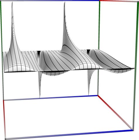
Left figure: real (“silver”) and imaginary (“gold”) part of the Jacobi theta function \(\theta_1(z, q)\). Camera angles are \(\theta=135^\circ\) and \(\phi = -12^\circ\), camera radius is -2.
See also Wikipedia [1424], MathWorld [1039], MathWorld [286], NIST [503], Ehrhardt [309] (3.2.13), Flint [818].
An example in Python
>>> from xlcalcnet import xreal
>>> xreal.JacobiTheta(1, 0.8, 0.5)
xreal('5.2359877559829887307E-1')
>>> xreal.JacobiTheta(2, 0.8, '0.51')
xreal('5.3518479027559984754E-1')
An example with real input for \(\theta_1(z,q)\):
>>> from xlcalcnet import dec, mpm, gmp, fpm, apm
>>> mpm.dps = 40; x = '3.8'; q = '0.7'
>>> \mathrm{d}x = dec.jtheta(1, x, q); mx = mpm.jtheta(1, x, q); gx = gmp.jtheta(1, x, q)
>>> fx = fpm.jtheta(1, x, q); ax = apm.jtheta(1, x, q)
>>> mpm.show([\mathrm{d}x, mx, gx, fx, ax])
dec:  -2.876223175938890139154258006053690969477E-1
mpm:  -2.876223175938890139154258006053690969477e-1
gmp:  -2.876223175938890139154258006053690969477E-01
fpm:  -2.87622317593889E-01
apm:  -2.876223175938890139154258006053690969480e-1 (-2.326e-35%)
An example with complex input for \(\theta_1(z,q)\):
>>> from xlcalcnet import dec, mpm, gmp, fpm, apm
>>> mpm.dps = 20; z = '11.0 + 3.0j'; q = '0.7 + 0.1j'
>>> \mathrm{d}z = dec.jtheta(1, z, q); mz = mpm.jtheta(1, z, q); gz = gmp.jtheta(1, z, q)
>>> fz = fpm.jtheta(1, z, q); az = apm.jtheta(1, z, q)
>>> mpm.show([\mathrm{d}z, mz, gz, fz, az], aligned=True)
dec: 1.3257637053506044723E+10              - 2.5508683032905869130E+9j
mpm: 1.3257637053506044723e+10              - 2.5508683032905869130e+9j
gmp: 1.3257637053506044723E+10              - 2.5508683032905869130E+09j
fpm: 1.32576370535060E+10                   - 2.55086830329060E+09j
apm: 1.3257637053506044630e+10 (4.315e-14%) - 2.5508683032905869160e+9 (-2.258e-13%)j
Jacobi theta function \(\theta_2(z, q)\)#
- ctx.jacobi_theta2(x, q)#
where
ctxismath53,ctxboostorctxflint.Returns the Jacobi theta function \(\displaystyle \theta_2(z,q) = 2 q^{1/4} \sum_{n=0}^{\infty} q^{n^{2\,} + n} \cos((2n+1)z)\)
Note: the Amath version needs to be adapted.
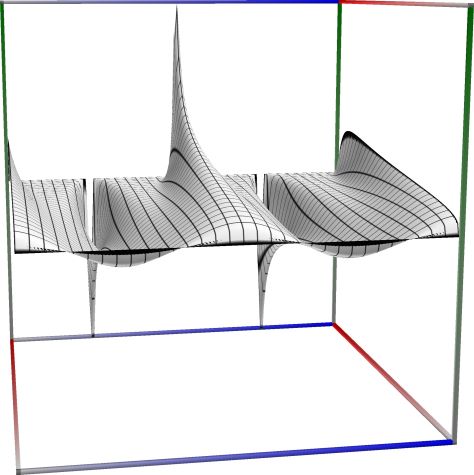
Left figure: real (“silver”) and imaginary (“gold”) part of the Jacobi theta function \(\theta_2(z, q)\). Camera angles are \(\theta=135^\circ\) and \(\phi = -12^\circ\), camera radius is -2.
See also Wikipedia [1424], MathWorld [1039], MathWorld [286], NIST [503], Ehrhardt [309] (3.2.13), Flint [818].
An example in Python
>>> from xlcalcnet import xreal
>>> xreal.JacobiTheta(1, 0.8, 0.5)
xreal('5.2359877559829887307E-1')
>>> xreal.JacobiTheta(2, 0.8, '0.51')
xreal('5.3518479027559984754E-1')
An example with real input for \(\theta_2(z,q)\):
>>> from xlcalcnet import dec, mpm, gmp, fpm, apm
>>> mpm.dps = 40; x = '3.8'; q = '0.7'
>>> \mathrm{d}x = dec.jtheta(2, x, q); mx = mpm.jtheta(2, x, q); gx = gmp.jtheta(2, x, q)
>>> fx = fpm.jtheta(2, x, q); ax = apm.jtheta(2, x, q)
>>> mpm.show([\mathrm{d}x, mx, gx, fx, ax])
dec:  -8.802379983271747955434299445752594240170E-1
mpm:  -8.802379983271747955434299445752594240170e-1
gmp:  -8.802379983271747955434299445752594240170E-01
fpm:  -8.80237998327175E-01
apm:  -8.802379983271747955434299445752594240180e-1 (-1.375e-35%)
An example with complex input for \(\theta_2(z,q)\):
>>> from xlcalcnet import dec, mpm, gmp, fpm, apm
>>> mpm.dps = 20; z = '11.0 + 3.0j'; q = '0.7 + 0.1j'
>>> \mathrm{d}z = dec.jtheta(2, z, q); mz = mpm.jtheta(2, z, q); gz = gmp.jtheta(2, z, q)
>>> fz = fpm.jtheta(2, z, q); az = apm.jtheta(2, z, q)
>>> mpm.show([\mathrm{d}z, mz, gz, fz, az], aligned=True)
dec: 2.6679401530814916188E+11              - 3.0867614993820689042E+11j
mpm: 2.6679401530814916188e+11              - 3.0867614993820689042e+11j
gmp: 2.6679401530814916188E+11              - 3.0867614993820689042E+11j
fpm: 2.66794015308149E+11                   - 3.08676149938205E+11j
apm: 2.6679401530814916130e+11 (4.123e-14%) - 3.0867614993820688890e+11 (-3.758e-14%)j
Jacobi theta function \(\theta_3(z, q)\)#
- ctx.jacobi_theta3(x, q)#
where
ctxismath53,ctxboostorctxflint.Returns the Jacobi theta function \(\displaystyle \theta_3(z,q) = 1 + 2 \sum_{n=1}^{\infty} q^{n^2\,} \cos(2 n z)\)
Note: the Amath version needs to be adapted.
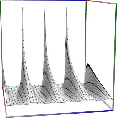
Left figure: real (“silver”) and imaginary (“gold”) part of the Jacobi theta function \(\theta_3(z, q)\). Camera angles are \(\theta=135^\circ\) and \(\phi = -12^\circ\), camera radius is -2.
See also Wikipedia [1424], MathWorld [1039], MathWorld [286], NIST [503], Ehrhardt [309] (3.2.13), Flint [818].
An example in Python
>>> from xlcalcnet import xreal
>>> xreal.JacobiTheta(1, 0.8, 0.5)
xreal('5.2359877559829887307E-1')
>>> xreal.JacobiTheta(2, 0.8, '0.51')
xreal('5.3518479027559984754E-1')
An example with real input for \(\theta_3(z,q)\):
>>> from xlcalcnet import dec, mpm, gmp, fpm, apm
>>> mpm.dps = 40; x = '3.8'; q = '0.7'
>>> \mathrm{d}x = dec.jtheta(3, x, q); mx = mpm.jtheta(3, x, q); gx = gmp.jtheta(3, x, q)
>>> fx = fpm.jtheta(3, x, q); ax = apm.jtheta(3, x, q)
>>> mpm.show([\mathrm{d}x, mx, gx, fx, ax])
dec:  8.802381825612654435491537366191521291923E-1
mpm:  8.802381825612654435491537366191521291923e-1
gmp:  8.802381825612654435491537366191521291923E-01
fpm:  8.80238182561266E-01
apm:  8.802381825612654435491537366191521291940e-1 (1.375e-35%)
An example with complex input for \(\theta_3(z,q)\):
>>> from xlcalcnet import dec, mpm, gmp, fpm, apm
>>> mpm.dps = 20; z = '11.0 + 3.0j'; q = '0.7 + 0.1j'
>>> \mathrm{d}z = dec.jtheta(3, z, q); mz = mpm.jtheta(3, z, q); gz = gmp.jtheta(3, z, q)
>>> fz = fpm.jtheta(3, z, q); az = apm.jtheta(3, z, q)
>>> mpm.show([\mathrm{d}z, mz, gz, fz, az], aligned=True)
dec: -2.6679401441538351941E+11               + 3.0867614546580330581E+11j
mpm: -2.6679401441538351941e+11               + 3.0867614546580330581e+11j
gmp: -2.6679401441538351941E+11               + 3.0867614546580330581E+11j
fpm: -2.66794014415383E+11                    + 3.08676145465801E+11j
apm: -2.6679401441538351880e+11 (-4.086e-14%) + 3.0867614546580330430e+11 (3.758e-14%)j
Jacobi theta function \(\theta_4(z, q)\)#
- ctx.jacobi_theta4(x, q)#
where
ctxismath53,ctxboostorctxflint.Returns the Jacobi theta function \(\displaystyle \theta_4(z,q) = 1 + 2 \sum_{n=1}^{\infty} (-q)^{n^2\,} \cos(2 n z)\)
Note: the Amath version needs to be adapted.
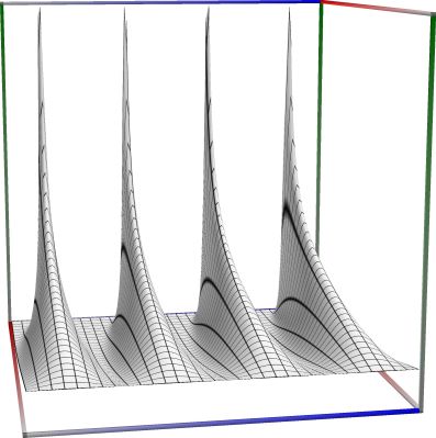
Left figure: real (“silver”) and imaginary (“gold”) part of the Jacobi theta function \(\theta_4(z, q)\). Camera angles are \(\theta=135^\circ\) and \(\phi = -12^\circ\), camera radius is -2.
See also Wikipedia [1424], MathWorld [1039], MathWorld [286], NIST [503], Ehrhardt [309] (3.2.13), Flint [818].
An example in Python
>>> from xlcalcnet import xreal
>>> xreal.JacobiTheta(1, 0.8, 0.5)
xreal('5.2359877559829887307E-1')
>>> xreal.JacobiTheta(2, 0.8, '0.51')
xreal('5.3518479027559984754E-1')
An example with real input for \(\theta_4(z,q)\):
>>> from xlcalcnet import dec, mpm, gmp, fpm, apm
>>> mpm.dps = 40; x = '3.8'; q = '0.7'
>>> \mathrm{d}x = dec.jtheta(4, x, q); mx = mpm.jtheta(4, x, q); gx = gmp.jtheta(4, x, q)
>>> fx = fpm.jtheta(4, x, q); ax = apm.jtheta(4, x, q)
>>> mpm.show([\mathrm{d}x, mx, gx, fx, ax])
dec:  2.876275982849924933190081281315277893390E-1
mpm:  2.876275982849924933190081281315277893390e-1
gmp:  2.876275982849924933190081281315277893390E-01
fpm:  2.87627598284992E-01
apm:  2.876275982849924933190081281315277893400e-1 (2.587e-35%)
An example with complex input for \(\theta_4(z,q)\):
>>> from xlcalcnet import dec, mpm, gmp, fpm, apm
>>> mpm.dps = 20; z = '11.0 + 3.0j'; q = '0.7 + 0.1j'
>>> \mathrm{d}z = dec.jtheta(4, z, q); mz = mpm.jtheta(4, z, q); gz = gmp.jtheta(4, z, q)
>>> fz = fpm.jtheta(4, z, q); az = apm.jtheta(4, z, q)
>>> mpm.show([\mathrm{d}z, mz, gz, fz, az], aligned=True)
dec: -1.3378357586306498825E+10               + 2.5798286002171674621E+9j
mpm: -1.3378357586306498825e+10               + 2.5798286002171674621e+9j
gmp: -1.3378357586306498825E+10               + 2.5798286002171674621E+09j
fpm: -1.33783575863064E+10                    + 2.57982860021718E+09j
apm: -1.3378357586306498730e+10 (-4.313e-14%) + 2.5798286002171674650e+9 (2.252e-13%)j