Factorials, Gamma and related functions

Gamma function, \(\Gamma(x)\)

ctx.gamma(x)

where ctx is math53, mathc53, ctxboost, ctxflint.

Returns the gamma function \(\displaystyle \Gamma(x) = \int_0^{\infty} t^{x-1} e^{-t} \, \mathrm{d}t\), for any real or complex \(x\) with \(\Re(x) > 0\) and for \(\Re(x) < 0\) by analytic continuation.

See also Wikipedia [1364], MathWorld [957], NIST [24], BoostMath [107], Ehrhardt [309] (3.5.1.1), Ehrhardt [309] (4.2.38), Flint [805], Flint [795], Mpmath [617].

\(\quad\) \(\quad\)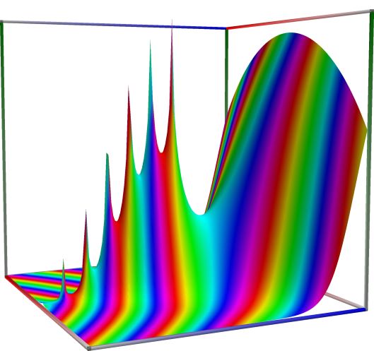

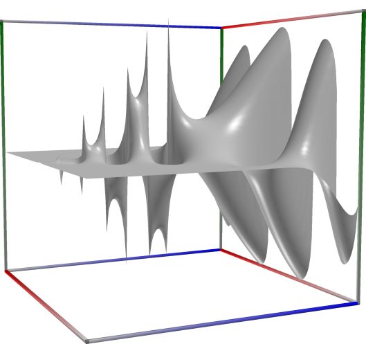
Left figure: real part of the Gamma function. Camera angles are \(\theta=135^\circ\) and \(\phi = -12^\circ\), camera radius is -2.

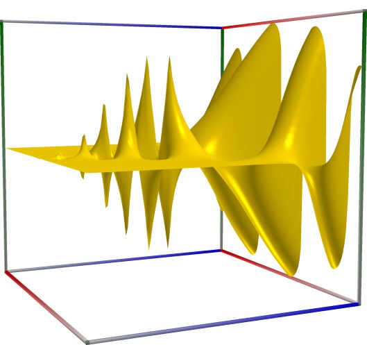
Middle figure: imaginary part of the Gamma function. Camera angles are \(\theta=135^\circ\) and \(\phi = -12^\circ\), camera radius is -2.

Right figure: absolute value of the Gamma function, with color-coded phase. Camera angles are \(\theta=135^\circ\) and \(\phi = -12^\circ\), camera radius is -2.

An example in Python

>>> from xlcalcnet import xreal
>>> xreal.Gamma(0.5)
xreal('5.2359877559829887307E-1')
>>> xreal.Gamma('0.51')
xreal('5.3518479027559984754E-1')

An example in Visual Basic

>>> from xlcalcnet import Gpr
>>> Gpr.Gamma(0.5)
Gpr('5.2359877559829887307E-1')
>>> Gpr.Gamma('0.51')
Gpr('5.3518479027559984754E-1')

An example with real input:

>>> from xlcalcnet import dec, mpm, ipm
>>> mpm.dps = 40; x = '10.5'
>>> \mathrm{d}x = dec.gamma(x); mx = mpm.gamma(x); ix = ipm.gamma(x)
>>> mpm.show([\mathrm{d}x, mx, ix])
dec:  1.133278388948785567334574165588892475560E+6
mpm:  1.133278388948785567334574165588892475560e+6
ipm:  1.133278388948785567334574165588892475560e+6 (1.062e-39%)

>>> from xlcalcnet import mpm, fpm, gmp, apm
>>> mpm.dps = 40; x = '10.5'
>>> fx = fpm.gamma(x); gx = gmp.gamma(x); ax = apm.gamma(x)
>>> mpm.show([fx, gx, ax])
fpm:  1.13327838894879E+06
gmp:  1.133278388948785567334574165588892475560E+06
apm:  1.133278388948785567334574165588892475560e+6 (1.062e-39%)

The following example with complex input shows that the relative error can be high in double precision:

>>> from xlcalcnet import dec, mpm, ipm
>>> mpm.dps = 20; z = '10.2 + 1.5E-2j'
>>> \mathrm{d}z = dec.gamma(z); mz = mpm.gamma(z); iz = ipm.gamma(z)
>>> mpm.show([\mathrm{d}z, mz, iz], aligned=True)
dec: 5.7016098526432799845E+5              + 1.9443478604345155482E+4j
mpm: 5.7016098526432799845e+5              + 1.9443478604345155482e+4j
ipm: 5.7016098526432799844e+5 (1.558e-18%) + 1.9443478604345155482e+4 (1.713e-18%)j

>>> from xlcalcnet import mpm, fpm, gmp, apm
>>> mpm.dps = 20; z = '10.2 + 1.5E-2j'
>>> fz = fpm.gamma(z); gz = gmp.gamma(z); az = apm.gamma(z)
>>> mpm.show([fz, gz, az], aligned=True)
fpm: 5.70160985264316E+05                  + 1.94434786043447E+04j
gmp: 5.7016098526432799845E+05             + 1.9443478604345155482E+04j
apm: 5.7016098526432799845e+5 (4.284e-18%) + 1.9443478604345155482e+4 (8.065e-18%)j

Arguments can also be large. Note that the gamma function grows very quickly:

>>> from xlcalcnet import mp
>>> mp.dps = 25; mp.pretty = True
>>> mp.dps = 15
>>> gamma(10**20)
1.9328495143101e+1956570551809674817225

Auxiliary function \(\Gamma(x+1)-1\)

ctx.real_gamma1pm1(z)

where ctx is math53, ctxcpp, ctxboost or ctxflint.

Returns \(\Gamma(1 + x) - 1\), accurate also for \(x\) near \(0\).

See also Wikipedia [1364], MathWorld [957], NIST [24], BoostMath [107], Ehrhardt [309] (3.5.1.2)., Flint [805], Flint [795].

Log-gamma function, \(\log\Gamma(x)\)

ctx.lgamma(x)

where ctx is math53, mathc53, ctxboost, ctxflint.

Returns the principal branch of the log-gamma function, \(\log|\Gamma(x)|\) for \(x \ne 0, -1, -2, \ldots\). If \(x<0\), the logarithmic form of the reflection formula is used.

See also: https://en.wikipedia.org/wiki/Gamma_function#Log-gamma_function

See also: https://mathworld.wolfram.com/LogGammaFunction.html

See also Wikipedia [1375], MathWorld [965], BoostMath [108], Ehrhardt [309] (3.5.1.5), Ehrhardt [309] (4.2.43), Flint [805], Flint [795], Mpmath [623].

Unlike \(\log(\Gamma(z))\), which has infinitely many complex branch cuts, the principal log-gamma function only has a single branch cut along the negative half-axis. The principal branch continuously matches the asymptotic Stirling expansion

\[\log \Gamma(z) \sim \frac{\log(2 \pi)}{2} + \left(z-\frac{1}{2}\right) \log(z) - z + O(z^{-1}).\]

The real parts of both functions agree, but their imaginary parts generally differ by \(2 n \pi\) for some \(n \in \mathbb{Z}\). They coincide for \(z \in \mathbb{R}, z > 0\).

\(\quad\) \(\quad\)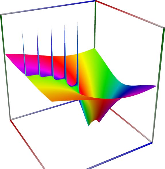

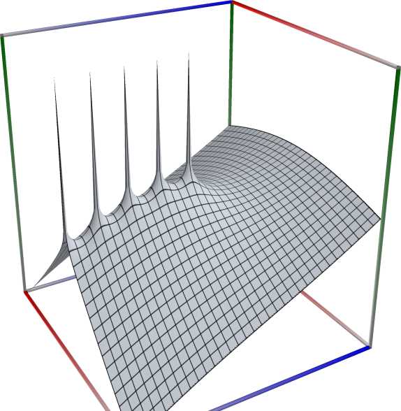
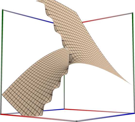
Left figure: real part of the LogGamma function. Camera angles are \(\theta=135^\circ\) and \(\phi = -12^\circ\), camera radius is -2.

Middle figure: imaginary part of the LogGamma function. Camera angles are \(\theta=135^\circ\) and \(\phi = -12^\circ\), camera radius is -2.

Right figure: absolute value of the LogGamma function, with color-coded phase. Camera angles are \(\theta=135^\circ\) and \(\phi = -12^\circ\), camera radius is -2.

An example in Python

>>> from xlcalcnet import xreal
>>> xreal.LogGamma(1.5)
xreal('5.2359877559829887307E-1')
>>> xreal.LogGamma('1.51')
xreal('5.3518479027559984754E-1')

An example in Visual Basic

>>> from xlcalcnet import Gpr
>>> Gpr.LogGamma(1.5)
Gpr('5.2359877559829887307E-1')
>>> Gpr.LogGamma('1.51')
Gpr('5.3518479027559984754E-1')

An example with real input:

>>> from xlcalcnet import dec, mpm, ipm
>>> mpm.dps = 40; x = '10.5'
>>> \mathrm{d}x = dec.loggamma(x); mx = mpm.loggamma(x); ix = ipm.loggamma(x)
>>> mpm.show([\mathrm{d}x, mx, ix])
dec:  1.394062521940376363316123788797184947980E+1
mpm:  1.394062521940376363316123788797184947980e+1
ipm:  1.394062521940376363316123788797184947980e+1 (6.588e-40%)

>>> from xlcalcnet import mpm, fpm, gmp, apm
>>> mpm.dps = 40; x = '10.5'
>>> fx = fpm.loggamma(x); gx = gmp.loggamma(x); ax = apm.loggamma(x)
>>> mpm.show([fx, gx, ax])
fpm:  1.39406252194038E+01
gmp:  1.394062521940376363316123788797184947980E+01
apm:  1.394062521940376363316123788797184947980e+1 (1.318e-39%)

The following example with complex input shows that the relative error can be high in double precision:

>>> from xlcalcnet import dec, mpm, ipm
>>> mpm.dps = 20; z = '10.2 + 1.5E-2j'
>>> \mathrm{d}z = dec.loggamma(z); mz = mpm.loggamma(z); iz = ipm.loggamma(z)
>>> mpm.show([\mathrm{d}z, mz, iz], aligned=True)
dec: 1.3254255156536136589E+1              + 3.4088524535204731293E-2j
mpm: 1.3254255156536136589e+1              + 3.4088524535204731293e-2j
ipm: 1.3254255156536136589e+1 (2.045e-19%) + 3.4088524535204731293e-2 (1.553e-19%)j

>>> from xlcalcnet import mpm, fpm, gmp, apm
>>> mpm.dps = 20; z = '10.2 + 1.5E-2j'
>>> fz = fpm.loggamma(z); gz = gmp.loggamma(z); az = apm.loggamma(z)
>>> mpm.show([fz, gz, az], aligned=True)
fpm: 1.32542551565361E+01                 + 3.40885245352047E-02j
gmp: 1.3254255156536136589E+01            + 3.4088524535204731293E-02j
apm: 1.3254255156536136589e+1 (4.09e-19%) + 3.4088524535204731293e-2 (6.989e-19%)j

Note the imaginary parts for negative arguments:

>>> from xlcalcnet import mpm
>>> mpm.dps = 25; mpm.pretty = True
>>> mpm.loggamma(-0.5); mpm.loggamma(-1.5); mpm.loggamma(-2.5)
(1.265512123484645396488946 - 3.141592653589793238462643j)
(0.8600470153764810145109327 - 6.283185307179586476925287j)
(-0.05624371649767405067259453 - 9.42477796076937971538793j)

Huge arguments are permitted:

>>> from xlcalcnet import dec, mpr, ivr, ivc
>>> ivr.dps = 25; ivr.pretty = True
>>> loggamma('1e3000')
6.906755278982137052053974e+3003
>>> loggamma('1e100000000000000000000')
2.302585092994045684007991e+100000000000000000020
>>> loggamma('1e300j')
(-1.570796326794896619231322e+300 + 6.897755278982137052053974e+302j)
>>> loggamma('1e3000j')
(-1.570796326794896619231322e+3000 + 6.906755278982137052053974e+3003j)

Reciprocal Gamma function, \(1/\Gamma(x)\)

ctx.rgamma(x)

where ctx is math53, mathc53, ctxboost, ctxflint.

Returns the reciprocal of gamma function \(x\), \(1/\Gamma(x)\), which is an entire function with simple zeros at the points \(x = 0\) and the negative integers.

See also Wikipedia [1374], MathWorld [967], Ehrhardt [309] (3.5.1.8), Ehrhardt [309] (4.2.51), Flint [805], Flint [795].

\(\quad\) \(\quad\)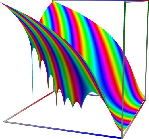

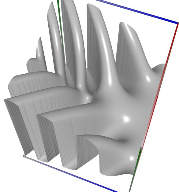
Left figure: real part of the RGamma function. Camera angles are \(\theta=135^\circ\) and \(\phi = -12^\circ\), camera radius is -2.

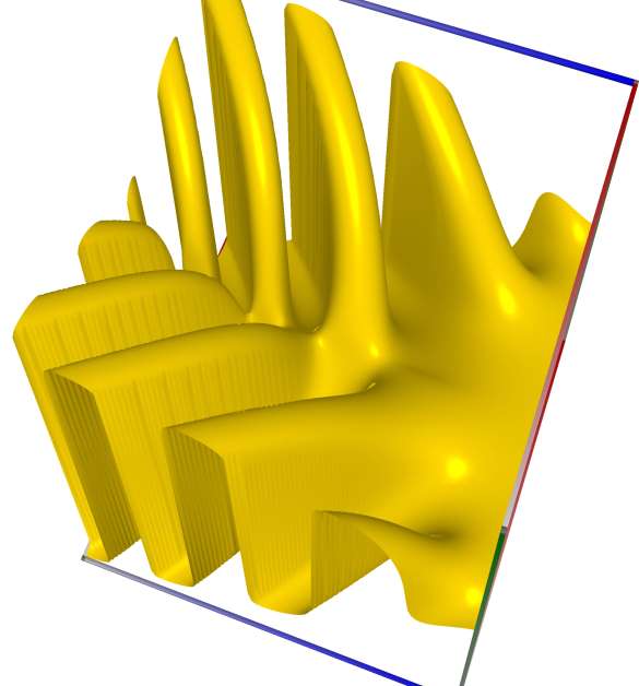
Middle figure: imaginary part of the RGamma function. Camera angles are \(\theta=135^\circ\) and \(\phi = -12^\circ\), camera radius is -2.

Right figure: absolute value of the RGamma function, with color-coded phase. Camera angles are \(\theta=135^\circ\) and \(\phi = -12^\circ\), camera radius is -2.

An example in Python

>>> from xlcalcnet import xreal
>>> xreal.RGamma(1)
1.0
>>> xreal.RGamma(4)
0.1666666666666666666666667
>>> xreal.RGamma(0); xreal.RGamma(-1)
0.0
0.0
>>> xreal.RGamma(1000)
2.485168143266784862783596e-2565
>>> xreal.RGamma('inf')
0.0

An example in Visual Basic

>>> from xlcalcnet import Gpr
>>> Gpr.RGamma(1)
1.0
>>> Gpr.RGamma(4)
0.1666666666666666666666667
>>> Gpr.RGamma(0); Gpr.RGamma(-1)
0.0
0.0
>>> Gpr.RGamma(1000)
0.0
>>> Gpr.RGamma('inf')
0.0

An example with real input:

>>> from xlcalcnet import dec, mpm, ipm
>>> mpm.dps = 40; x = '10.5'
>>> \mathrm{d}x = dec.rgamma(x); mx = mpm.rgamma(x); ix = ipm.rgamma(x)
>>> mpm.show([\mathrm{d}x, mx, ix])
dec:  8.823957200203800905509402624256928377655E-7
mpm:  8.823957200203800905509402624256928377655e-7
ipm:  8.823957200203800905509402624256928377655e-7 (1.861e-39%)

>>> from xlcalcnet import mpm, fpm, gmp, apm
>>> mpm.dps = 40; x = '10.5'
>>> fx = fpm.rgamma(x); gx = gmp.rgamma(x); ax = apm.rgamma(x)
>>> mpm.show([fx, gx, ax])
fpm:  8.82395720020380E-07
gmp:  8.823957200203800905509402624256928377655E-07
apm:  8.823957200203800905509402624256928377655e-7 (6.203e-40%)

The following example with complex input shows that the relative error can be high in double precision:

>>> from xlcalcnet import dec, mpm, ipm
>>> mpm.dps = 20; z = '10.2 + 1.5E-2j'
>>> \mathrm{d}z = dec.rgamma(z); mz = mpm.rgamma(z); iz = ipm.rgamma(z)
>>> mpm.show([\mathrm{d}z, mz, iz], aligned=True)
dec: 1.7518533332561467304E-6              - 5.9741237445991417084E-8j
mpm: 1.7518533332561467304e-6              - 5.9741237445991417084e-8j
ipm: 1.7518533332561467304e-6 (4.749e-18%) - 5.9741237445991417085e-8 (-4.902e-18%)j

>>> from xlcalcnet import mpm, fpm, gmp, apm
>>> mpm.dps = 20; z = '10.2 + 1.5E-2j'
>>> fz = fpm.rgamma(z); gz = gmp.rgamma(z); az = apm.rgamma(z)
>>> mpm.show([fz, gz, az], aligned=True)
fpm: 1.75185333325618E-06                  - 5.97412374459925E-08j
gmp: 1.7518533332561467304E-06             - 5.9741237445991417084E-08j
apm: 1.7518533332561467304e-6 (4.242e-18%) - 5.9741237445991417084e-8 (-7.521e-18%)j

This function evaluates to zero at the poles of the gamma function, \(z = 0, -1, -2, \ldots\).

>>> from xlcalcnet import dec, mpr, ivr, ivc
>>> ivr.dps = 25; ivr.pretty = True
>>> rgamma(1)
1.0
>>> rgamma(4)
0.1666666666666666666666667
>>> rgamma(0); rgamma(-1)
0.0
0.0
>>> rgamma(1000)
2.485168143266784862783596e-2565
>>> rgamma(inf)
0.0

Factorial, \(x!\)

ctx.factorial(x)

where ctx is math53, ctxboost or ctxflint.

Returns \(x!\), the factorial of \(x\). For integers \(x \ge 0\), we have \(x! = 1 \cdot 2 \cdots (x-1) \cdot x\) and for real or complex \(x\) we have \(x! = \Gamma(x+1)\).

See also Wikipedia [1362], MathWorld [955], BoostMath [105], Ehrhardt [309] (3.5.4.1), Flint [805], Flint [795], Mpmath [615].

An example in Python

>>> from xlcalcnet import xreal
>>> xreal.Factorial(3)
xreal('5.2359877559829887307E-1')
>>> xreal.Factorial('0.51')
xreal('5.3518479027559984754E-1')

An example in Visual Basic

>>> from xlcalcnet import Gpr
>>> Gpr.Factorial(3)
Gpr('5.2359877559829887307E-1')
>>> Gpr.Factorial('0.51')
Gpr('5.3518479027559984754E-1')

Double factorial, \(x!!\)

ctx.double_factorial(x)

where ctx is math53, ctxboost or ctxflint.

Returns \(x!!\), the double factorial of \(x\).

\[\begin{split}n!!=\begin{cases} 1 \cdot 3 \cdot 5 \cdots n & \text{ if } n \text{ is odd.}\\ 2 \cdot 4 \cdot 6 \cdots n & \text{ if } n \text{ is even.} \end{cases}\end{split}\]

and more generally by

\[x!! = 2^{x/2} \left(\frac{\pi}{2}\right)^{(\cos(\pi x)-1)/4} \Gamma\left(\frac{x}{2}+1\right).\]

See also Wikipedia [1382], MathWorld [991], BoostMath [124], Ehrhardt [309] (3.5.4.2), Flint [805], Flint [795], Mpmath [636].

See also http://dlmf.nist.gov/5.4.E2

An example in Python

>>> from xlcalcnet import xreal
>>> xreal.DFactorial(3)
xreal('5.2359877559829887307E-1')
>>> xreal.DFactorial('0.51')
xreal('5.3518479027559984754E-1')

An example in Visual Basic

>>> from xlcalcnet import Gpr
>>> Gpr.DFactorial(3)
Gpr('5.2359877559829887307E-1')
>>> Gpr.DFactorial('0.51')
Gpr('5.3518479027559984754E-1')

Rising factorial \(a^{\overline{n}} = (a)_n\)

ctx.rising_factorial(a, n)

where ctx is math53, ctxboost or ctxflint.

Returns the rising factorial , \(\displaystyle a^{\overline{n}} = (a)_n = a (a+1) \cdots (a+n-1) = \frac{\Gamma(a+n)}{\Gamma(a)}\,\), where the rightmost expression is valid for nonintegral \(n\). By convention \((a)_0 = 1\). Note that in Wikipedia [1363], the Pochhammer symbol \((a)_n\) is used for the falling factorial (as is common in combinatorics), whereas in this manual we follow the convention in MathWorld [968], Abramowitz and Stegun. [4], BoostMath [116], Ehrhardt [309], and the literature of special functions (in particular the hypergeometric functions), using it for the rising factorial.

If \(a\) or \(a + n\) are negative integers or zero special care must be taken: If only \(a\) is a negative integer then the result is zero. If \(a + n\) is also a negative integer then the Pochhammer symbol is computed from the limiting form of the \(\Gamma\) reflection formula \(\displaystyle (a)_n = (-1)^n \frac{\Gamma(1-a)}{\Gamma(1-a-n)}\), and otherwise the function is undefined.

See also Wikipedia [1363], MathWorld [968], BoostMath [116], Ehrhardt [309] (3.5.4.6), Flint [805], Flint [795], Mpmath [628].

An example in Python

>>> from xlcalcnet import xreal
>>> xreal.Pochhammer(13, 7)
xreal('5.2359877559829887307E-1')
>>> xreal.RisingFactorial(12.6, '4.51')
xreal('5.3518479027559984754E-1')

An example in Visual Basic

>>> from xlcalcnet import Gpr
>>> Gpr.Pochhammer(13, 7)
Gpr('5.2359877559829887307E-1')
>>> Gpr.RisingFactorial(12.6, '4.51')
Gpr('5.3518479027559984754E-1')

An example with real input:

>>> from xlcalcnet import dec, mpm, ipm
>>> mpm.dps = 40; x = '20.4'; n = '10.4'
>>> \mathrm{d}x = dec.rf(x, n); mx = mpm.rf(x, n); ix = ipm.rf(x, n)
>>> mpm.show([\mathrm{d}x, mx, ix])
dec:  3.343372973979018889554680008371771979653E+14
mpm:  3.343372973979018889554680008371771979652e+14
ipm:  3.343372973979018889554680008371771979655e+14 (1.836e-37%)

>>> from xlcalcnet import mpm, fpm, gmp, apm
>>> mpm.dps = 40; x = '20.4'; n = '10.4'
>>> fx = fpm.rf(x, n); gx = gmp.rf(x, n); ax = apm.rf(x, n)
>>> mpm.show([fx, gx, ax])
fpm:  3.34337297397901E+14
gmp:  3.343372973979018889554680008371771979652E+14
apm:  3.343372973979018889554680008371771979654e+14 (3.73e-37%)

The following example with complex input shows that the relative error can be high in double precision:

>>> from xlcalcnet import dec, mpm, ipm
>>> mpm.dps = 20; z = '20.2 + 1.5E-2j'; n = '10.7 + 2.3E-1j'
>>> \mathrm{d}z = dec.rf(z, n); mz = mpm.rf(z, n); iz = ipm.rf(z, n)
>>> mpm.show([\mathrm{d}z, mz, iz], aligned=True)
dec: 5.9977312704618499868E+14              + 6.0755212828478581691E+14j
mpm: 5.9977312704618499868e+14              + 6.0755212828478581692e+14j
ipm: 5.9977312704618499868e+14 (2.178e-17%) + 6.0755212828478581692e+14 (2.292e-17%)j

>>> from xlcalcnet import mpm, fpm, gmp, apm
>>> mpm.dps = 20; z = '20.2 + 1.5E-2j'; n = '10.7 + 2.3E-1j'
>>> fz = fpm.rf(z, n); gz = gmp.rf(z, n); az = apm.rf(z, n)
>>> mpm.show([fz, gz, az], aligned=True)
fpm: 5.99773127046176E+14                   + 6.07552128284776E+14j
gmp: 5.9977312704618499868E+14              + 6.0755212828478581692E+14j
apm: 5.9977312704618499868e+14 (4.245e-17%) + 6.0755212828478581692e+14 (4.442e-17%)j

Evaluation is supported for arbitrary arguments:

>>> from xlcalcnet import mp
>>> mp.dps = 25; mp.pretty = True
>>> mp.rf(2+3j, 5.5)
(-7202.03920483347 - 3777.58810701527j)

Falling factorial, \((a)^{\underline{n}} = (a-n+1)^{\overline{n}}\)

ctx.falling_factorial(a, n)

where ctx is math53, ctxboost or ctxflint.

Returns the falling factorial of \(a\) and \(n\), \(\displaystyle a^{\underline{n}} = a (a-1) \cdots (a-n+1) = \frac{\Gamma(a+1)}{\Gamma(a+1-n)}\,\), where the rightmost expression is valid for nonintegral \(n\).

The falling factorial \((a)^{\underline{n}}\) is related to the rising factorial \((a)^{\overline{n}}\) by \((a)^{\underline{n}} = (a-n+1)^{\overline{n}}\).

See also Wikipedia [1363], MathWorld [956], BoostMath [106], Mpmath [616].

An example in Python

>>> from xlcalcnet import xreal
>>> xreal.FallingFactorial(13, 7)
xreal('5.2359877559829887307E-1')
>>> xreal.FallingFactorial(12.6, '4.51')
xreal('5.3518479027559984754E-1')

An example in Visual Basic

>>> from xlcalcnet import Gpr
>>> Gpr.FallingFactorial(13, 7)
Gpr('5.2359877559829887307E-1')
>>> Gpr.FallingFactorial(12.6, '4.51')
Gpr('5.3518479027559984754E-1')

Ratio of gamma functions, \(\Gamma(a)/\Gamma(b)\)

ctx.real_gamma_ratio(a, b)

where ctx is math53, ctxcpp, ctxboost or ctxflint.

This functions returns the ratio of gamma functions in the form

\[\frac{\Gamma(a)}{\Gamma(b)}\]

See also BoostMath [132], Ehrhardt [309] (3.5.5).

An example with real input:

>>> from xlcalcnet import dec, mpm, ipm
>>> mpm.dps = 40; a = '20.4'; b = '10.4'
>>> \mathrm{d}x = dec.gamma_ratio(a, b); mx = mpm.gamma_ratio(a, b); ix = ipm.gamma_ratio(a, b)
>>> mpm.show([\mathrm{d}x, mx, ix])
dec:  4.450005383343493349376000000000000000000E+11
mpm:  4.450005383343493349376000000000000000000e+11
ipm:  4.450005383343493349376000000000000000001e+11 (7.871e-38%)

>>> from xlcalcnet import mpm, fpm, gmp, apm
>>> mpm.dps = 40; a = '20.4'; b = '10.4'
>>> fx = fpm.gamma_ratio(a, b); gx = gmp.gamma_ratio(a, b); ax = apm.gamma_ratio(a, b)
>>> mpm.show([fx, gx, ax])
fpm:  4.45000538334346E+11
gmp:  4.450005383343493349376000000000000000000E+11
apm:  4.450005383343493349376000000000000000000e+11 (2.049e-37%)

Gamma-delta ratio, \(\Gamma(a)/\Gamma(a + \delta)\)

ctx.real_gamma_delta_ratio(x, delta)

where ctx is math53, ctxcpp, ctxboost or ctxflint.

Returns the tgamma_ratio function of z and m. See also BoostMath [132].

Returns \(\Gamma(x)/\Gamma(x+d)\), accurate even for \(|d| << |x|\).

This functions returns the ratio of gamma functions in the form

\[\frac{\Gamma(a)}{\Gamma(a+\delta)}\]

Note that the result is calculated accurately even when \(\delta\) is small compared to \(a\): indeed even if \(a+\delta \approx a\). The function is typically used when \(a\) is large and \(\delta\) is very small.

Note: ctxboost.TgammaDeltaRatio(x, d)

Returns \(\displaystyle \frac{\Gamma(x)}{\Gamma(x+d)}\,\), accurate also for \(|d| \ll |x|\).

See also BoostMath [132], Ehrhardt [309] (3.5.5).

An example with real input:

>>> from xlcalcnet import dec, mpm, ipm
>>> mpm.dps = 40; a = '2000.4'; d = '0.0004'
>>> \mathrm{d}z = dec.gamma_delta_ratio(a, d); mz = mpm.gamma_delta_ratio(a, d)
>>> iz = ipm.gamma_delta_ratio(a, d); fz = fpm.gamma_delta_ratio(a, d)
>>> gz = gmp.gamma_delta_ratio(a, d); az = apm.gamma_delta_ratio(a, d)
>>> mpm.show([\mathrm{d}x, mx, ix, fx, gx, ax])
dec:  9.969642761288672131226497458238654348190E-1
mpm:  9.969642761288672131226497458238654347429e-1
ipm:  9.969642761288672131226497458238654348320e-1 (2.681e-35%)
fpm:  9.96964276128867E-01
gmp:  9.969642761288672131226497458238654347429E-01
apm:  9.969642761288672131226497458238654348405e-1 (3.693e-35%)

Beta function, \(B(a,b) = \Gamma(a)\Gamma(b)/\Gamma(a + b)\)

ctx.beta(a, b)

where ctx is math53, ctxboost or ctxflint.

Returns the beta dunction \(\displaystyle B(a,b) = \frac{\Gamma(a)\Gamma(b)}{\Gamma(a + b}\)

Binomial coefficient, \({}_nC_k = (k \cdot B(k, n-k+1))^{-1}\)

ctx.binomial(n, k)

where ctx is math53, ctxboost or ctxflint.

Returns the binomial coefficient of \(n\) and \(k\), \(\displaystyle {}_nC_k = {n \choose k} = \frac{n!}{k!(n-k)!}\), for \(k \geq 0\). More generally, the binomial coefficient is a well-defined function of arbitrary real or complex \(n\) and \(k\), via the gamma function.

\[{}_{n}C_{k} = {n \choose k} = \frac{n!}{k!(n-k)!} = \frac{\Gamma(n+1)}{\Gamma(k+1)\Gamma(n-k+1)} = \frac{1}{k \cdot B(k, n-k+1)}.\]

See also Wikipedia [1359], MathWorld [954], NIST [509], BoostMath [102], Ehrhardt [309] (3.5.4.4), Flint [805], Flint [795], Mpmath [614].

An example in Python

>>> from xlcalcnet import xreal
>>> xreal.Binomial(13, 7)
xreal('5.2359877559829887307E-1')
>>> xreal.Binomial(12.6, '4.51')
xreal('5.3518479027559984754E-1')

An example in Visual Basic

>>> from xlcalcnet import Gpr
>>> Gpr.Binomial(13, 7)
Gpr('5.2359877559829887307E-1')
>>> Gpr.Binomial(12.6, '4.51')
Gpr('5.3518479027559984754E-1')