Trigonometric functions, in radians

For a general introduction to trigonometric functions, see Wikipedia [1353], NIST [517].

Sine, \(\sin(x)\)

ctx.sin(x)

where ctx is ctx_pm (see Python contexts for details), ctx53, ctxcpp, ctxflint (see .NET contexts for details). The corresponding ctx python lists are ctxlistreal and ctxlistcplx.

Returns the sine of \(x\), \(\sin(x)\). See also Wikipedia [1350], MathWorld [947], NIST [517], Ehrhardt [309] (4.2.55), Flint [812], Flint [802], Mpmath [584].

The sine can be defined as \(\displaystyle \sin(x) = x - \frac{x^3}{3!} + \frac{x^5}{5!} - \frac{x^7}{7!} + \cdots = \sum_{n=0}^\infty \frac{(-1)^n}{(2n+1)!}x^{2n+1}\).

The complex sine can be expressed in terms of related real functions:

\[\sin(z) = \sin(x+iy) = \frac {e^{iz}-e^{-iz}}{2i} = \sin(x) \cosh(y) + i \cos(x) \sinh(y).\]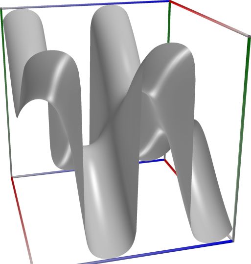

\(\quad\) \(\quad\)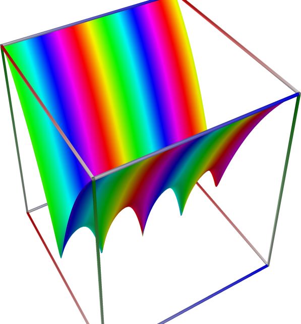

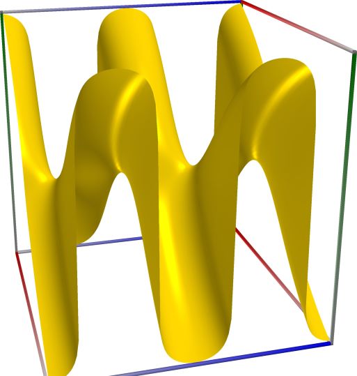
3D wpf plot: real part (left figure), imaginary part (middle figure) and absolute value with color-coded phase (right figure) of the complex sine function \(z = \sin(x + iy)\), with \(-6 \le x \le 6\) (blue axis), \(-6 \le y \le 6\) (red axis), \(-10 \le z \le 10\) (green axis). Function values are loglog-transformed.

An example with real input:

>>> from xlcalcnet import *
>>> x = -5.1; dps = 90
>>> for ctx in ctxlistreal: print(ctx.fmtname + ': ' + ctx.fmt(ctx.sin(x)))
    fpm:  0.925814682327732
    mpm:  0.925814682327732296946146247544863312509403016355603948797054551932281847236566889436906375
    dpm:  0.925814682327732296946146247544863312509403016355603948797054551932281847236566889436906375
    ipm: [0.92581468232773229694614624754486331250940301635560394879705455193228184723656688943690637503659,
          0.9258146823277322969461462475448633125094030163556039487970545519322818472365668894369063755275]
    gpm:  0.92581468232773229694614624754486331250940301635560394879705455193228184723656688943690637504
    apm: [0.92581468232773229694614624754486331250940301635560394879705455193228184723656688943690638 +/- 5.10e-90]
 math53:  0.925814682327732
  sreal:  0.9258147
  dreal:  0.925814682327732
  ereal:  0.92581468232773229699
  qreal:  0.925814682327732296946146247544863
  oreal:  0.92581468232773229694614624754486331250940301635560394879705455193228186
  mreal:  0.925814682327732296946146247544863312509403016355603948797054551932281847236566889436906376
 sflint:  0.9258147
 dflint:  0.925814682327732
 eflint:  0.92581468232773229699
 qflint:  0.925814682327732296946146247544863
 oflint:  0.92581468232773229694614624754486331250940301635560394879705455193228185
 mflint:  0.925814682327732296946146247544863312509403016355603948797054551932281847236566889436906376
 aflint: [0.925814682327732296946146247544863312509403016355603948797054551932281847236566889436906375 +/- 9.57e-91]

An example with complex input, using C#-style formatting for complex numbers for the result

>>> from xlcalcnet import *
>>> x = -5.1+2j; gui.setdps(50)
>>> for ctx in [fpm, mpm, cmath53, qcplx]: print(ctx.fmtname + ': ' + ctx.fmt(ctx.sin(x)))
    fpm:  (3.48309600859536, 1.37087251009309)
    mpm:  (3.483096008595355530539519132049601874260208157133, 1.3708725100930962119067139658774871514235754109441)
cmath53:  (3.48309600859536, 1.37087251009309)
  qcplx:  (3.4830960085953555305395191320496, 1.37087251009309621190671396587749)

An example with the same complex input as above, showing only the real part of the result:

>>> from xlcalcnet import *
>>> x = -5.1+2j; gui.setdps(90)
>>> for ctx in gui.ctxlistcplx: print(ctx.fmtname + ': ' +  ctx.realctx.fmt(ctx.real(ctx.sin(x))))
    fpm:  3.48309600859536
    mpm:  3.48309600859535553053951913204960187426020815713299066103565188114779116680123268271030781
    dpm:  3.48309600859535553053951913204960187426020815713299066103565188114779116680123268271030781
    ipm: [3.4830960085953555305395191320496018742602081571329906610356518811477911668012326827103078127848,
          3.4830960085953555305395191320496018742602081571329906610356518811477911668012326827103078147484]
    gpm:  3.4830960085953555305395191320496018742602081571329906610356518811477911668012326827103078133
    apm: [3.48309600859535553053951913204960187426020815713299066103565188114779116680123268271030781 +/- 6.64e-90]
cmath53:  3.48309600859536
  scplx:  3.483096
  dcplx:  3.48309600859536
  ecplx:  3.4830960085953555309
  qcplx:  3.4830960085953555305395191320496
  ocplx:  3.4830960085953555305395191320496018742602081571329906610356518811477912
  mcplx:  3.48309600859535553053951913204960187426020815713299066103565188114779116680123268271030782
sflintc:  3.483096
dflintc:  3.48309600859536
eflintc:  3.4830960085953555307
qflintc:  3.4830960085953555305395191320496
oflintc:  3.4830960085953555305395191320496018742602081571329906610356518811477912
mflintc:  3.48309600859535553053951913204960187426020815713299066103565188114779116680123268271030782
aflintc: [3.48309600859535553053951913204960187426020815713299066103565188114779116680123268271030781 +/- 8.22e-90]

An example with the same complex input as above, showing only the imaginary part of the result:

>>> from xlcalcnet import *
>>> x = -5.1+2j; gui.setdps(90)
>>> for ctx in gui.ctxlistcplx: print(ctx.fmtname + ': ' +  ctx.realctx.fmt(ctx.imag(ctx.sin(x))))
    fpm:  1.37087251009309
    mpm:  1.37087251009309621190671396587748715142357541094412916331060531052891362760947942650352236
    dpm:  1.37087251009309621190671396587748715142357541094412916331060531052891362760947942650352236
    ipm: [1.3708725100930962119067139658774871514235754109441291633106053105289136276094794265035223541435,
          1.3708725100930962119067139658774871514235754109441291633106053105289136276094794265035223575799]
    gpm:  1.3708725100930962119067139658774871514235754109441291633106053105289136276094794265035223576
    apm: [1.37087251009309621190671396587748715142357541094412916331060531052891362760947942650352235 +/- 7.68e-90]
cmath53:  1.37087251009309
  scplx:  1.370872
  dcplx:  1.37087251009309
  ecplx:  1.3708725100930962117
  qcplx:  1.37087251009309621190671396587749
  ocplx:  1.3708725100930962119067139658774871514235754109441291633106053105289136
  mcplx:  1.37087251009309621190671396587748715142357541094412916331060531052891362760947942650352235
sflintc:  1.370872
dflintc:  1.37087251009309
eflintc:  1.3708725100930962116
qflintc:  1.37087251009309621190671396587749
oflintc:  1.3708725100930962119067139658774871514235754109441291633106053105289136
mflintc:  1.37087251009309621190671396587748715142357541094412916331060531052891362760947942650352235
aflintc: [1.37087251009309621190671396587748715142357541094412916331060531052891362760947942650352235 +/- 7.29e-90]

Cosine, \(\cos(x)\)

ctx.cos(x)

where ctx is math53, mathc53, ctxcpp, ctxflint.

Returns the cosine of \(x\), \(\cos(x)\). See also Wikipedia [1353], MathWorld [932], NIST [517], Ehrhardt [309] (4.2.19), Flint [812], Flint [802], Mpmath [567].

The cosine can be defined as \(\displaystyle \cos(x) = 1 - \frac{x^2}{2!} + \frac{x^4}{4!} - \frac{x^6}{6!} + \cdots = \sum_{n=0}^\infty \frac{(-1)^n}{(2n)!}x^{2n}\).

The complex cosine can be expressed in terms of related real functions:

\[\cos(z) = \cos(x+iy) = \frac {e^{ix}+e^{-ix}}{2} = \cos(x) \cosh(y) - i \sin(x) \sinh(y).\]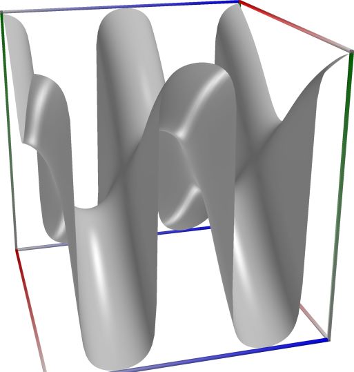

\(\quad\) 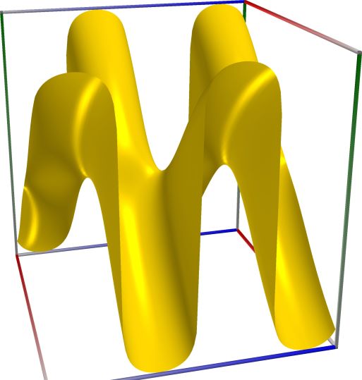\(\quad\)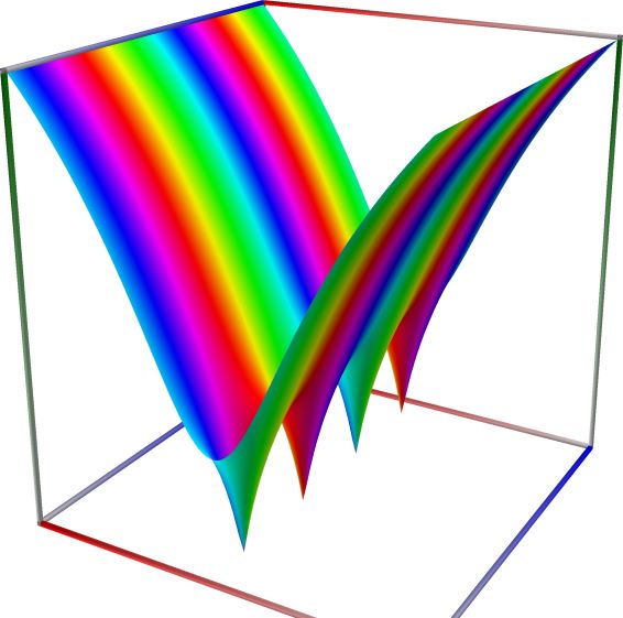

Left figure: real part of the Cosine function. Camera angles are \(\theta=135^\circ\) and \(\phi = -12^\circ\), camera radius is -2.

Middle figure: imaginary part of the Cosine function. Camera angles are \(\theta=135^\circ\) and \(\phi = -12^\circ\), camera radius is -2.

Right figure: absolute value of the Cosine function, with color-coded phase. Camera angles are \(\theta=135^\circ\) and \(\phi = -12^\circ\), camera radius is -2.

An example in Python

>>> from xlcalcnet import xreal
>>> xreal.Cos(0.5)
xreal('5.2359877559829887307E-1')
>>> xreal.Cos('0.51')
xreal('5.3518479027559984754E-1')

An example in Visual Basic

>>> from xlcalcnet import Gpr
>>> Gpr.Cos(0.5)
Gpr('5.2359877559829887307E-1')
>>> Gpr.Cos('0.51')
Gpr('5.3518479027559984754E-1')

An example with real input:

>>> from xlcalcnet import dec, mpm, ipm
>>> mpm.dps = 40; x = '1.57079632679489'
>>> \mathrm{d}x = dec.cos(x); mx = mpm.cos(x); ix = ipm.cos(x)
>>> mpm.show([\mathrm{d}x, mx, ix])
dec:  6.619231321691639751442098584651351473054E-15
mpm:  6.619231321691639751442098575708073666164e-15
ipm:  6.619231321691639751442098587187510685913e-15 (1.734e-25%)

>>> from xlcalcnet import mpm, fpm, gmp, apm
>>> mpm.dps = 40; x = '1.57079632679489'
>>> fx = fpm.cos(x); gx = gmp.cos(x); ax = apm.cos(x)
>>> mpm.show([fx, gx, ax])
fpm:  6.72257048770831E-15
gmp:  6.619231321691639751442098575708073666164E-15
apm:  6.619231321691639751442098584676383837843e-15 (1.768e-25%)

The following example with complex input shows that the relative error can be high in double precision:

>>> from xlcalcnet import dec, mpm, ipm
>>> mpm.dps = 20; z = '3.14159265358979 + 1.5E+2j'
>>> \mathrm{d}z = dec.cos(z); mz = mpm.cos(z); iz = ipm.cos(z)
>>> mpm.show([\mathrm{d}z, mz, iz], aligned=True)
dec: -6.9685479033318984866E+64             - 2.2567382063567230055E+50j
mpm: -6.9685479033318984866e+64             - 2.2567375654278714043e+50j
ipm: -6.9685479033318984866e+64 (-6.4e-20%) - 2.2567387459458051327e+50 (-5.231e-5%)j

>>> from xlcalcnet import mpm, fpm, gmp, apm
>>> mpm.dps = 20; z = '3.14159265358979 + 1.5E+2j'
>>> fz = fpm.cos(z); gz = gmp.cos(z); az = apm.cos(z)
>>> mpm.show([fz, gz, az], aligned=True)
fpm: -6.96854790333190E+64                  - 2.25159995138029E+50j
gmp: -6.9685479033318984866E+64             - 2.2567375654278714043E+50j
apm: -6.9685479033318984866e+64 (-6.4e-20%) - 2.2567382294692091265e+50 (-5.406e-5%)j

Tangent, \(\tan(x)\)

ctx.tan(x)

where ctx is math53, mathc53, ctxcpp, ctxflint.

Returns the tangent of \(x\), \(\tan(x)\). See also Wikipedia [1353], MathWorld [948], NIST [517], Ehrhardt [309] (4.2.61), Flint [812], Flint [802], Mpmath [607].

The tangent can be defined in terms of related functions as \(\displaystyle \tan(x) = \frac{\sin(x)}{\cos(x)}\).

The tangent function is singular at \(x = (n+1/2)\pi\), but tan(x) always returns a finite result since \((n+1/2)\pi\) cannot be represented exactly using floating-point arithmetic.

The complex tangent can be expressed in terms of related real functions:

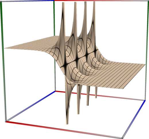
\[\tan(z) = \tan(x+iy) = \frac{\sin(z)}{\cos(z)} = \frac{\sin(2x) + i \sinh(2y)}{\cos(2x) + i \cosh(2y)}\]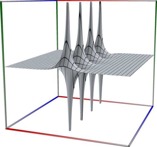

\(\quad\) \(\quad\)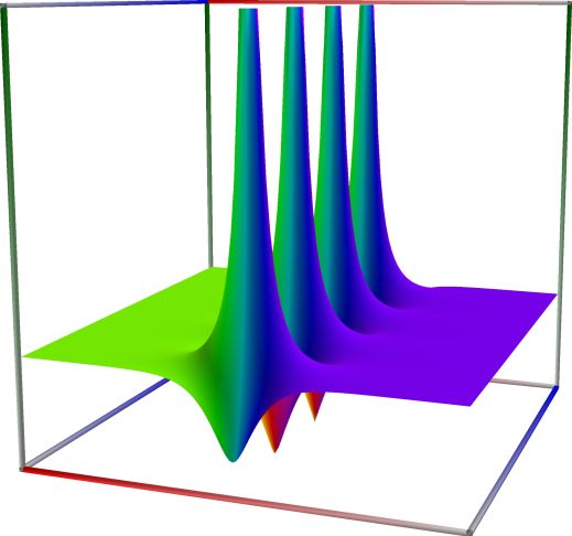

Left figure: real part of the Tangent function. Camera angles are \(\theta=135^\circ\) and \(\phi = -12^\circ\), camera radius is -2.

Middle figure: imaginary part of the Tangent function. Camera angles are \(\theta=135^\circ\) and \(\phi = -12^\circ\), camera radius is -2.

Right figure: absolute value of the Tangent function, with color-coded phase. Camera angles are \(\theta=135^\circ\) and \(\phi = -12^\circ\), camera radius is -2.

An example in Python

>>> from xlcalcnet import xreal
>>> xreal.Tan(0.5)
xreal('5.2359877559829887307E-1')
>>> xreal.Tan('0.51')
xreal('5.3518479027559984754E-1')

An example in Visual Basic

>>> from xlcalcnet import Gpr
>>> Gpr.Tan(0.5)
Gpr('5.2359877559829887307E-1')
>>> Gpr.Tan('0.51')
Gpr('5.3518479027559984754E-1')

An example with real input:

>>> from xlcalcnet import dec, mpm, ipm
>>> mpm.dps = 40; x = '1.57079632679489'
>>> \mathrm{d}x = dec.tan(x); mx = mpm.tan(x); ix = ipm.tan(x)
>>> mpm.show([\mathrm{d}x, mx, ix])
dec:  1.510749438115173197484743336377677954945E+14
mpm:  1.510749438115173197484743338418859364845e+14
ipm:  1.510749438115173197484743335798834140673e+14 (1.734e-25%)

>>> from xlcalcnet import mpm, fpm, gmp, apm
>>> mpm.dps = 40; x = '1.57079632679489'
>>> fx = fpm.tan(x); gx = gmp.tan(x); ax = apm.tan(x)
>>> mpm.show([fx, gx, ax])
fpm:  1.48752623989354E+14
gmp:  1.510749438115173197484743338418859364845E+14
apm:  1.510749438115173197484743336371964655059e+14 (1.767e-25%)

The following example with complex input shows that the relative error can be high in double precision:

>>> from xlcalcnet import dec, mpm, ipm
>>> mpm.dps = 20; z = '1.57079632679489 + 0.001j'
>>> \mathrm{d}z = dec.tan(z); mz = mpm.tan(z); iz = ipm.tan(z)
>>> mpm.show([\mathrm{d}z, mz, iz], aligned=True)
dec: 6.6192291152816404696E-9            + 1.0000003333333111111E+3j
mpm: 6.6192285676675710077e-9            + 1.0000003333333111111e+3j
ipm: 6.6192294147002359176e-9 (1.28e-5%) + 1.0000003333333111111e+3 (6.505e-19%)j

>>> from xlcalcnet import mpm, fpm, gmp, apm
>>> mpm.dps = 20; z = '1.57079632679489 + 0.001j'
>>> fz = fpm.tan(z); gz = gmp.tan(z); az = apm.tan(z)
>>> mpm.show([fz, gz, az], aligned=True)
fpm: 6.72256824685193E-09                + 1.00000033333331E+03j
gmp: 6.6192285676675710076E-09           + 1.0000003333333111111E+03j
apm: 6.6192291235327573548e-9 (1.32e-5%) + 1.0000003333333111111e+3 (1.301e-19%)j

From mpmath:

>>> from xlcalcnet import  mp
>>> iv.tan([0,2])  # Interval includes a singularity
[-inf, +inf]

Cotangent, \(\cot(x)\)

ctx.cot(x)

where ctx is math53, mathc53, ctxcpp, ctxflint.

Returns the cotangent of \(x\), \(\mathrm{cot}(x)\). See also Wikipedia [1353], MathWorld [933], NIST [517], Ehrhardt [309] (4.2.21), Flint [812], Flint [802], Mpmath [587].

The cotangent can be expressed in terms of related functions as \(\displaystyle \cot(x) = \frac{\cos(x)}{\sin(x)}\).

This cotangent function is singular at \(x = n \pi\), but with the exception of the point \(x = 0\), cot(x) returns a finite result since \(n \pi\) cannot be represented exactly using floating-point arithmetic.

The complex cotangent can be expressed in terms of related real functions:

\[\cot(z) = \cot(x+iy) = \frac{\cos(z)}{\sin(z)} = \frac{\cos(2x) + i \cosh(2y)}{\sin(2x) + i \sinh(2y)}\]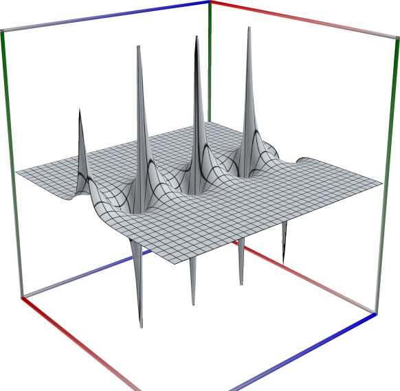

\(\quad\) \(\quad\)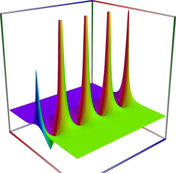

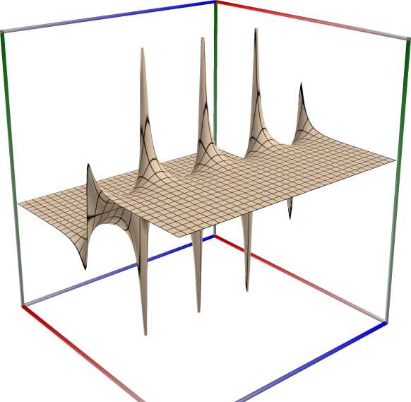
Left figure: real part of the Cotangent function. Camera angles are \(\theta=135^\circ\) and \(\phi = -12^\circ\), camera radius is -2.

Middle figure: imaginary part of the Cotangent function. Camera angles are \(\theta=135^\circ\) and \(\phi = -12^\circ\), camera radius is -2.

Right figure: absolute value of the Cotangent function, with color-coded phase. Camera angles are \(\theta=135^\circ\) and \(\phi = -12^\circ\), camera radius is -2.

An example in Python

>>> from xlcalcnet import xreal
>>> xreal.Cot(0.5)
xreal('5.2359877559829887307E-1')
>>> xreal.Cot('0.51')
xreal('5.3518479027559984754E-1')

An example in Visual Basic

>>> from xlcalcnet import Gpr
>>> Gpr.Cot(0.5)
Gpr('5.2359877559829887307E-1')
>>> Gpr.Cot('0.51')
Gpr('5.3518479027559984754E-1')

An example with real input:

>>> from xlcalcnet import dec, mpm, ipm
>>> mpm.dps = 40; x = '1.57079632679489'
>>> \mathrm{d}x = dec.cot(x); mx = mpm.cot(x); ix = ipm.cot(x)
>>> mpm.show([\mathrm{d}x, mx, ix])
dec:  6.619231321691639751442098584796359712623E-15
mpm:  6.619231321691639751442098575853081905733e-15
ipm:  6.619231321691639751442098587332518925482e-15 (1.734e-25%)

>>> from xlcalcnet import mpm, fpm, gmp, apm
>>> mpm.dps = 40; x = '1.57079632679489'
>>> fx = fpm.cot(x); gx = gmp.cot(x); ax = apm.cot(x)
>>> mpm.show([fx, gx, ax])
fpm:  6.72257048770831E-15
gmp:  6.619231321691639751442098575853081905733E-15
apm:  6.619231321691639751442098584821392051071e-15 (1.768e-25%)

The following example with complex input shows that the relative error can be high in double precision:

>>> from xlcalcnet import dec, mpm, ipm
>>> mpm.dps = 20; z = '1.57079632679489 + 0.001j'
>>> \mathrm{d}z = dec.cot(z); mz = mpm.cot(z); iz = ipm.cot(z)
>>> mpm.show([\mathrm{d}z, mz, iz], aligned=True)
dec: 6.6192247024647308782E-15            - 9.9999966666679999995E-4j
mpm: 6.6192241548510264921e-15            - 9.9999966666679999995e-4j
ipm: 6.6192250018831267140e-15 (1.28e-5%) - 9.9999966666679999995e-4 (-4.963e-19%)j

>>> from xlcalcnet import mpm, fpm, gmp, apm
>>> mpm.dps = 20; z = '1.57079632679489 + 0.001j'
>>> fz = fpm.cot(z); gz = gmp.cot(z); az = apm.cot(z)
>>> mpm.show([fz, gz, az], aligned=True)
fpm: 6.72256376514230E-15                 - 9.99999666666800E-04j
gmp: 6.6192241548510264921E-15            - 9.9999966666679999995E-04j
apm: 6.6192247107158422627e-15 (1.32e-5%) - 9.9999966666679999995e-4 (-1.654e-19%)j

Cosecant, \(\mathrm{csc}(x)\)

ctx.csc(x)

where ctx is math53, mathc53, ctxcpp or ctxflint.

Returns the cosecant of \(x\), \(\mathrm{csc}(x)\). See also Wikipedia [1353], MathWorld [931], NIST [517], Ehrhardt [309] (4.2.23), Flint [812], Flint [802], Mpmath [586].

The cosecant can be expressed in terms of related functions as \(\displaystyle \csc(x) = \frac{1}{\sin(x)}\).

The cosecant function is singular at \(x = n \pi\), but with the exception of the point \(x = 0\), csc(x) returns a finite result since \(n \pi\) cannot be represented exactly using floating-point arithmetic.

The complex cosecant can be expressed in terms of related real functions:

\[\csc(z) = \csc(x+iy) = \frac{1}{\sin(z)} = \frac {2i}{e^{ix}-e^{-ix}} = \frac {1} {\sin(x) \cosh(y) + i \cos(x) \sinh(y)}.\]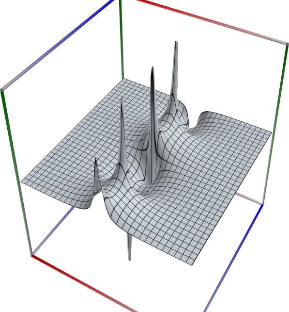

\(\quad\) 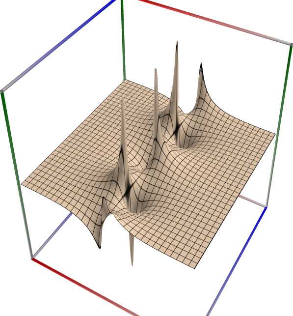\(\quad\)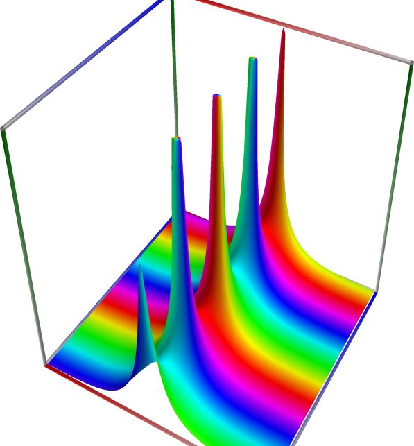

Left figure: real part of the Cosecant function. Camera angles are \(\theta=135^\circ\) and \(\phi = -12^\circ\), camera radius is -2.

Middle figure: imaginary part of the Cosecant function. Camera angles are \(\theta=135^\circ\) and \(\phi = -12^\circ\), camera radius is -2.

Right figure: absolute value of the Cosecant function, with color-coded phase. Camera angles are \(\theta=135^\circ\) and \(\phi = -12^\circ\), camera radius is -2.

An example in Python

>>> from xlcalcnet import xreal
>>> xreal.Csc(0.5)
xreal('5.2359877559829887307E-1')
>>> xreal.Csc('0.51')
xreal('5.3518479027559984754E-1')

An example in Visual Basic

>>> from xlcalcnet import Gpr
>>> Gpr.Csc(0.5)
Gpr('5.2359877559829887307E-1')
>>> Gpr.Csc('0.51')
Gpr('5.3518479027559984754E-1')

An example with real input:

>>> from xlcalcnet import dec, mpm, ipm
>>> mpm.dps = 40; x = '3.14159265358979'
>>> \mathrm{d}x = dec.csc(x); mx = mpm.csc(x); ix = ipm.csc(x)
>>> mpm.show([\mathrm{d}x, mx, ix])
dec:  3.087884932201293574786585956747166309734E+14
mpm:  3.087884932201293574786585940687795154700e+14
ipm:  3.087884932201293574786585962579158129574e+14 (7.089e-25%)

>>> from xlcalcnet import mpm, fpm, gmp, apm
>>> mpm.dps = 40; x = '3.14159265358979'
>>> fx = fpm.csc(x); gx = gmp.csc(x); ax = apm.csc(x)
>>> mpm.show([fx, gx, ax])
fpm:  3.09493162808962E+14
gmp:  3.087884932201293574786585940687795154700E+14
apm:  3.087884932201293574786585956422212234890e+14 (7.222e-25%)

The following example with complex input shows that the relative error can be high in double precision:

>>> from xlcalcnet import dec, mpm, ipm
>>> mpm.dps = 20; z = '1.57079632679489 + 1.5E+2j'
>>> \mathrm{d}z = dec.csc(z); mz = mpm.csc(z); iz = ipm.csc(z)
>>> mpm.show([\mathrm{d}z, mz, iz], aligned=True)
dec: 1.4350191946328820840E-65              - 9.4987240003426845058E-80j
mpm: 1.4350191946328820840e-65              - 9.4987232145057216312e-80j
ipm: 1.4350191946328820840e-65 (5.605e-20%) - 9.4987244300142594276e-80 (-1.28e-5%)j

>>> from xlcalcnet import mpm, fpm, gmp, apm
>>> mpm.dps = 20; z = '1.57079632679489 + 1.5E+2j'
>>> fz = fpm.csc(z); gz = gmp.csc(z); az = apm.csc(z)
>>> mpm.show([fz, gz, az], aligned=True)
fpm: 1.43501919463288E-65                   - 9.64701768713396E-80j
gmp: 1.4350191946328820840E-65              - 9.4987232145057216313E-80j
apm: 1.4350191946328820840e-65 (5.605e-20%) - 9.4987240121831995601e-80 (-1.326e-5%)j

Secant, \(\mathrm{sec}(x)\)

ctx.sec(x)

where ctx is math53, mathc53, ctxcpp or ctxflint.

Returns the secant of \(x\), \(\mathrm{sec}(x)\). See also Wikipedia [1353], MathWorld [946], NIST [517], Ehrhardt [309] (4.2.53), Flint [812], Flint [802], Mpmath [606].

The secant can be expressed in terms of related functions as \(\displaystyle \sec(x) = \frac{1}{\cos(x)}\).

The secant function is singular at \(x = (n+1/2)\pi\), but sec(x) always returns a finite result since \((n+1/2)\pi\) cannot be represented exactly using floating-point arithmetic.

The complex secant can be expressed in terms of related real functions:

\[\sec(z) = \sec(x+iy) = \frac{1}{\cos(z)} = \frac {2}{e^{ix}+e^{-ix}} = \frac {1} {\cos(x) \cosh(y) - i \sin(x) \sinh(y)}.\]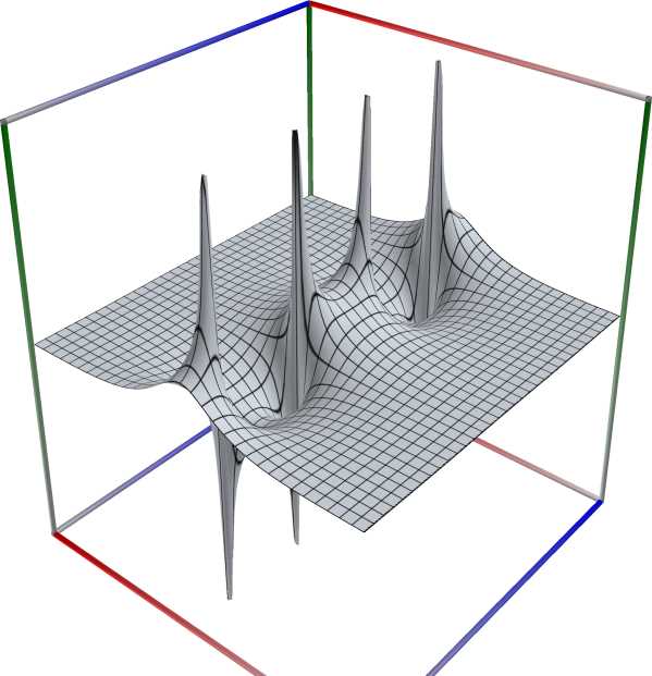

\(\quad\) 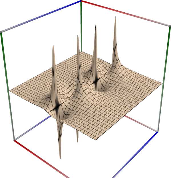\(\quad\)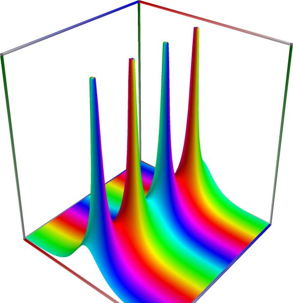

Left figure: real part of the Secant function. Camera angles are \(\theta=135^\circ\) and \(\phi = -12^\circ\), camera radius is -2.

Middle figure: imaginary part of the Secant function. Camera angles are \(\theta=135^\circ\) and \(\phi = -12^\circ\), camera radius is -2.

Right figure: absolute value of the Secant function, with color-coded phase. Camera angles are \(\theta=135^\circ\) and \(\phi = -12^\circ\), camera radius is -2.

An example in Python

>>> from xlcalcnet import xreal
>>> xreal.Sec(0.5)
xreal('5.2359877559829887307E-1')
>>> xreal.Sec('0.51')
xreal('5.3518479027559984754E-1')

An example in Visual Basic

>>> from xlcalcnet import Gpr
>>> Gpr.Sec(0.5)
Gpr('5.2359877559829887307E-1')
>>> Gpr.Sec('0.51')
Gpr('5.3518479027559984754E-1')

An example with real input:

>>> from xlcalcnet import dec, mpm, ipm
>>> mpm.dps = 40; x = '1.57079632679489'
>>> \mathrm{d}x = dec.sec(x); mx = mpm.sec(x); ix = ipm.sec(x)
>>> mpm.show([\mathrm{d}x, mx, ix])
dec:  1.510749438115173197484743336410774111554E+14
mpm:  1.510749438115173197484743338451955521454e+14
ipm:  1.510749438115173197484743335831930297281e+14 (1.734e-25%)

>>> from xlcalcnet import mpm, fpm, gmp, apm
>>> mpm.dps = 40; x = '1.57079632679489'
>>> fx = fpm.sec(x); gx = gmp.sec(x); ax = apm.sec(x)
>>> mpm.show([fx, gx, ax])
fpm:  1.48752623989354E+14
gmp:  1.510749438115173197484743338451955521454E+14
apm:  1.510749438115173197484743336405060807289e+14 (1.767e-25%)

The following example with complex input shows that the relative error can be high in double precision:

>>> from xlcalcnet import dec, mpm, ipm
>>> mpm.dps = 20; z = '3.14159265358979 + 1.5E+2j'
>>> \mathrm{d}z = dec.sec(z); mz = mpm.sec(z); iz = ipm.sec(z)
>>> mpm.show([\mathrm{d}z, mz, iz], aligned=True)
dec: -1.4350191946328820840E-65               + 4.6472560543565481719E-80j
mpm: -1.4350191946328820840e-65               + 4.6472547345045256263e-80j
ipm: -1.4350191946328820840e-65 (-5.605e-20%) + 4.6472571655216012191e-80 (5.231e-5%)j

>>> from xlcalcnet import mpm, fpm, gmp, apm
>>> mpm.dps = 20; z = '3.14159265358979 + 1.5E+2j'
>>> fz = fpm.sec(z); gz = gmp.sec(z); az = apm.sec(z)
>>> mpm.show([fz, gz, az], aligned=True)
fpm: -1.43501919463288E-65                    + 4.63667494819155E-80j
gmp: -1.4350191946328820840E-65               + 4.6472547345045256263E-80j
apm: -1.4350191946328820840e-65 (-5.605e-20%) + 4.6472561019516306473e-80 (5.401e-5%)j

Cardinal sine, \(\mathrm{sinc}(x)\)

ctx.sinc(x)

where ctx is math53, mathc53, ctxcpp, ctxflint.

Returns the cardinal sine of x. See also Wikipedia [1397], MathWorld [1007], BoostMath [133], Flint [812], Flint [802], Mpmath [632].

sinc(x) computes the unnormalized sinc function, defined as \(\displaystyle \mathrm{sinc}(x) = \begin{cases} \sin(x)/x, & \mbox{if } x \ne 0 \\ 1, & \mbox{if } x = 0. \end{cases}\)

An example in Python

>>> from xlcalcnet import xreal
>>> xreal.Sinc(0.5)
xreal('5.2359877559829887307E-1')
>>> xreal.Sinc('0.51')
xreal('5.3518479027559984754E-1')

An example in Visual Basic

>>> from xlcalcnet import Gpr
>>> Gpr.Sinc(0.5)
Gpr('5.2359877559829887307E-1')
>>> Gpr.Sinc('0.51')
Gpr('5.3518479027559984754E-1')

An example with real input:

>>> from xlcalcnet import dec, mpm, ipm
>>> mpm.dps = 40; x = '0.0000001'
>>> \mathrm{d}x = dec.sinc(x); mx = mpm.sinc(x); ix = ipm.sinc(x)
>>> mpm.show([\mathrm{d}x, mx, ix])
dec:  9.999999999999983333333333333341666666667E-1
mpm:  9.999999999999983333333333333341666666667e-1
ipm:  9.999999999999983333333333333341666666667e-1 (2.87e-39%)

>>> from xlcalcnet import mpm, fpm, gmp, apm
>>> mpm.dps = 40; x = '0.0000001'
>>> fx = fpm.sinc(x); gx = gmp.sinc(x); ax = apm.sinc(x)
>>> mpm.show([fx, gx, ax])
fpm:  9.99999999999998E-01
gmp:  9.999999999999983333333333333341666666667E-01
apm:  9.999999999999983333333333333341666666667e-1 (5.74e-40%)

The following example with complex input shows that the relative error can be high in double precision:

>>> from xlcalcnet import dec, mpm, ipm
>>> mpm.dps = 20; z = '0.0000001 + 0.001j'
>>> \mathrm{d}z = dec.sinc(z); mz = mpm.sinc(z); iz = ipm.sinc(z)
>>> mpm.show([\mathrm{d}z, mz, iz], aligned=True)
dec: 1.0000001666666733333E+0              - 3.3333336666666752381E-11j
mpm: 1.0000001666666733333e+0              - 3.3333336666666752360e-11j
ipm: 1.0000001666666733333e+0 (5.082e-19%) - 3.3333336666666640784e-11 (-1.199e-12%)j

>>> from xlcalcnet import mpm, fpm, gmp, apm
>>> mpm.dps = 20; z = '0.0000001 + 0.001j'
>>> fz = fpm.sinc(z); gz = gmp.sinc(z); az = apm.sinc(z)
>>> mpm.show([fz, gz, az], aligned=True)
fpm: 1.00000016666667E+00                 - 3.33333366590436E-11j
gmp: 1.0000001666666733333E+00            - 3.3333336666666773989E-11j
apm: 1.0000001666666733333e+0 (8.47e-20%) - 3.3333336666666751169e-11 (-2.592e-12%)j