Inverse trigonometric functions, in radians

For a general introduction to inverse trigonometric functions, see Wikipedia [1366], NIST [512].

Inverse sine, \(\mathrm{asin}(x)\)

ctx.asin(x)

where ctx is math53, mathc53, ctxcpp, ctxflint.

Returns the inverse sine of \(x\), \(\mathrm{asin}(x)\). See also Wikipedia [1366], MathWorld [944], NIST [512], Ehrhardt [309] (4.2.13), Mpmath [604].

The inverse sine can be expressed in terms of the inverse tangent as \(\displaystyle \mathrm{asin}(x) = \mathrm{atan}\left(\frac{x}{\sqrt{1-x^2}} \right)\). The domain is the open interval \((-1, 1)\). We have \(\sin(\mathrm{asin}(x)) = x\) for all \(x\), but \(\mathrm{asin}(\sin(x)) = x\) only for \(-\pi/2 < x < \pi/2\).

The inverse sine can be expressed in terms of related functions (with the principal-branch log and square root):

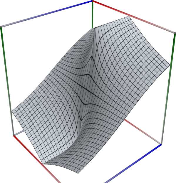
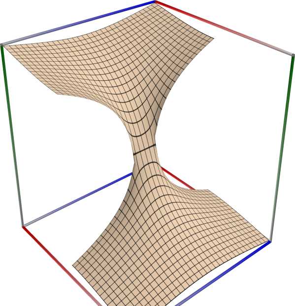
\[\mathrm{asin}(z) = -i \log\left(iz + \sqrt{1-z^2} \right)\]

The inverse sine has two branch points: \(x = \pm 1\).The branch cuts are placed along the line segments \((-\infty, -1)\) and \((+1, +\infty)\). Since \(-1 \le \sin(x) \le 1\) for real \(x\), the inverse sine is real-valued only for \(-1 \le x \le 1\). On this interval, it is defined to be a monotonically increasing function assuming values between \(-\pi/2\) and \(\pi/2\).

\(\quad\) \(\quad\)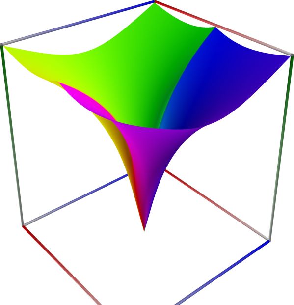

Left figure: real part of the Inverse Sine function. Camera angles are \(\theta=135^\circ\) and \(\phi = -12^\circ\), camera radius is -2.

Middle figure: imaginary part of the Inverse Sine function. Camera angles are \(\theta=135^\circ\) and \(\phi = -12^\circ\), camera radius is -2.

Right figure: absolute value of the Inverse Sine function, with color-coded phase. Camera angles are \(\theta=135^\circ\) and \(\phi = -12^\circ\), camera radius is -2.

An example in Python

>>> from xlcalcnet import xreal
>>> xreal.Asin(0.5)
xreal('5.2359877559829887307E-1')
>>> xreal.Asin('0.51')
xreal('5.3518479027559984754E-1')

An example in Visual Basic

>>> from xlcalcnet import Gpr
>>> Gpr.Asin(0.5)
Gpr('5.2359877559829887307E-1')
>>> Gpr.Asin('0.51')
Gpr('5.3518479027559984754E-1')

An example with real input:

>>> from xlcalcnet import dec, mpm, ipm
>>> mpm.dps = 40; x = '1'
>>> \mathrm{d}x = dec.asin(x); mx = mpm.asin(x); ix = ipm.asin(x)
>>> mpm.show([\mathrm{d}x, mx, ix])
dec:  1.570796326794896619231321691639751442099E+0
mpm:  1.570796326794896619231321691639751442099e+0
ipm:  1.570796326794896619231321691639751442099e+0 (7.308e-40%)

>>> from xlcalcnet import mpm, fpm, gmp, apm
>>> mpm.dps = 40; x = '1'
>>> fx = fpm.asin(x); gx = gmp.asin(x); ax = apm.asin(x)
>>> mpm.show([fx, gx, ax])
fpm:  1.57079632679490E+00
gmp:  1.570796326794896619231321691639751442099E+00
apm:  1.570796326794896619231321691639751442099e+0 (1.462e-39%)

The following example with complex input shows that the relative error can be high in double precision:

>>> from xlcalcnet import dec, mpm, ipm
>>> mpm.dps = 20; z = '1 + 1.5E-2j'
>>> \mathrm{d}z = dec.asin(z); mz = mpm.asin(z); iz = ipm.asin(z)
>>> mpm.show([\mathrm{d}z, mz, iz], aligned=True)
dec: 1.4484754471355477567E+0              + 1.2262706126402998997E-1j
mpm: 1.4484754471355477567e+0              + 1.2262706126402998997e-1j
ipm: 1.4484754471355477567e+0 (1.754e-19%) + 1.2262706126402998997e-1 (1.295e-18%)j

>>> from xlcalcnet import mpm, fpm, gmp, apm
>>> mpm.dps = 20; z = '1 + 1.5E-2j'
>>> fz = fpm.asin(z); gz = gmp.asin(z); az = apm.asin(z)
>>> mpm.show([fz, gz, az], aligned=True)
fpm: 1.44847544713555E+00                  + 1.22627061264030E-01j
gmp: 1.4484754471355477567E+00             + 1.2262706126402998997E-01j
apm: 1.4484754471355477567e+0 (5.848e-20%) + 1.2262706126402998997e-1 (1.727e-19%)j

\(\mathrm{asin}(z)\) is defined so as to be a proper inverse function of \(\sin(\theta)\) for \(-\pi/2 < \theta < \pi/2\). We have \(\sin(\sin^{-1}(x)) = x\) for all \(x\), but \(\sin^{-1}(\sin(x)) = x\) only for \(-\pi/2 < \Re[x] < \pi/2\):

>>> from xlcalcnet import dec, mpr, ivr, ivc
>>> ivr.dps = 25; ivr.pretty = True
>>> for x in [1, 10, -1, 1+3j, -2+3j]:
...     print("%s %s" % (chop(sin(asin(x))), asin(sin(x))))
...
1.0 1.0
10.0 -0.5752220392306202846120698
-1.0 -1.0
(1.0 + 3.0j) (1.0 + 3.0j)
(-2.0 + 3.0j) (-1.141592653589793238462643 - 3.0j)

Inverse cosine, \(\mathrm{acos}(x)\)

ctx.acos(x)

where ctx is math53, mathc53, ctxcpp, ctxflint.

Returns the inverse cosine of \(x\), \(\mathrm{acos}(x)\). See also Wikipedia [1366], MathWorld [941], NIST [512], Ehrhardt [309] (4.2.3), Flint [809], Flint [799], Mpmath [595].

The inverse cosine can be expressed in terms of the inverse tangent as \(\displaystyle \mathrm{acos}(x) = \mathrm{atan}\left(\frac{\sqrt{1-x^2}}{x} \right)\). The domain is the open interval \((-1, 1)\). We have \(\cos(\mathrm{acos}(x)) = x\) for all \(x\), but \(\mathrm{acos}(\cos(x)) = x\) only for \(0 \le x < \pi\).

The inverse cosine can be expressed in terms of related functions (with the principal-branch log and square root):

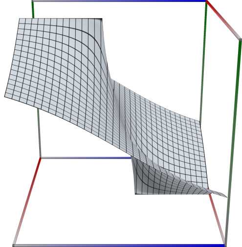
\[\mathrm{acos}(z) = \frac{\pi}{2} + i \log\left(iz + \sqrt{1-z^2} \right)\]

The inverse cosine has two branch points: \(x = \pm 1\).The branch cuts are placed along the line segments \((-\infty, -1)\) and \((+1, +\infty)\).

Since \(-1 \le \cos(x) \le 1\) for real \(x\), the inverse cosine is real-valued only for \(-1 \le x \le 1\), where it is a monotonically decreasing function assuming values between \(+\pi\) and \(0\).

\(\quad\) \(\quad\)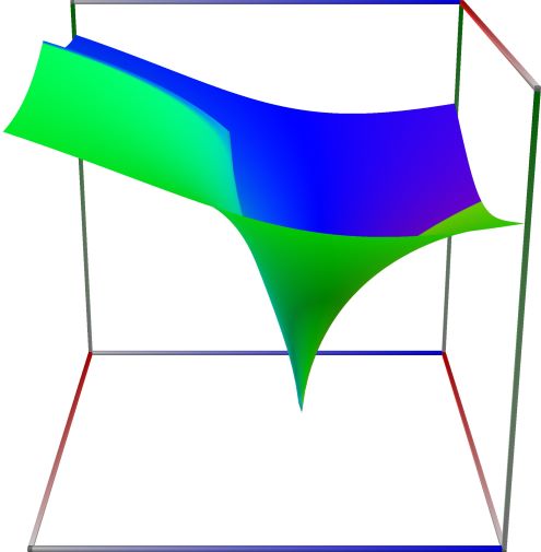

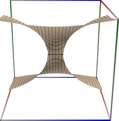
Left figure: real part of the Inverse Cosine function. Camera angles are \(\theta=135^\circ\) and \(\phi = -12^\circ\), camera radius is -2.

Middle figure: imaginary part of the Inverse Cosine function. Camera angles are \(\theta=135^\circ\) and \(\phi = -12^\circ\), camera radius is -2.

Right figure: absolute value of the Inverse Cosine function, with color-coded phase. Camera angles are \(\theta=135^\circ\) and \(\phi = -12^\circ\), camera radius is -2.

An example in Python

>>> from xlcalcnet import xreal
>>> xreal.Acos(0.5)
xreal('5.2359877559829887307E-1')
>>> xreal.Acos('0.51')
xreal('5.3518479027559984754E-1')

An example in Visual Basic

>>> from xlcalcnet import Gpr
>>> Gpr.Acos(0.5)
Gpr('5.2359877559829887307E-1')
>>> Gpr.Acos('0.51')
Gpr('5.3518479027559984754E-1')

An example with real input:

>>> from xlcalcnet import dec, mpm, ipm
>>> mpm.dps = 40; x = '0.5'
>>> \mathrm{d}x = dec.acos(x); mx = mpm.acos(x); ix = ipm.acos(x)
>>> mpm.show([\mathrm{d}x, mx, ix])
dec:  1.047197551196597746154214461093167628066E+0
mpm:  1.047197551196597746154214461093167628066e+0
ipm:  1.047197551196597746154214461093167628066e+0 (1.096e-39%)

>>> from xlcalcnet import mpm, fpm, gmp, apm
>>> mpm.dps = 40; x = '0.5'
>>> fx = fpm.acos(x); gx = gmp.acos(x); ax = apm.acos(x)
>>> mpm.show([fx, gx, ax])
fpm:  1.04719755119660E+00
gmp:  1.047197551196597746154214461093167628066E+00
apm:  1.047197551196597746154214461093167628066e+0 (1.096e-39%)

The following example with complex input shows that the relative error can be high in double precision:

>>> from xlcalcnet import dec, mpm, ipm
>>> mpm.dps = 20; z = '0.5 + 1.5E-2j'
>>> \mathrm{d}z = dec.acos(z); mz = mpm.acos(z); iz = ipm.acos(z)
>>> mpm.show([\mathrm{d}z, mz, iz], aligned=True)
dec: 1.0472841234408009862E+0              - 1.7318776682711839316E-2j
mpm: 1.0472841234408009862e+0              - 1.7318776682711839316e-2j
ipm: 1.0472841234408009862e+0 (8.088e-20%) - 1.7318776682711839316e-2 (-4.967e-18%)j

>>> from xlcalcnet import mpm, fpm, gmp, apm
>>> mpm.dps = 20; z = '0.5 + 1.5E-2j'
>>> fz = fpm.acos(z); gz = gmp.acos(z); az = apm.acos(z)
>>> mpm.show([fz, gz, az], aligned=True)
fpm: 1.04728412344080E+00                  - 1.73187766827118E-02j
gmp: 1.0472841234408009862E+00             - 1.7318776682711839316E-02j
apm: 1.0472841234408009862e+0 (1.618e-19%) - 1.7318776682711839316e-2 (-3.821e-19%)j

\(\mathrm{acos}(z)\) is defined so as to be a proper inverse function of \(\cos(\theta)\) for \(0 \le \theta < \pi\). We have \(\cos(\cos^{-1}(x)) = z\) for all \(z\), but \(\cos^{-1}(\cos(z)) = z\) only for \(0 \le \Re[x] < \pi\):

>>> from xlcalcnet import dec, mpr, ivr, ivc
>>> ivr.dps = 25; ivr.pretty = True
>>> for x in [1, 10, -1, 2+3j, 10+3j]:
...     print("%s %s" % (cos(acos(x)), acos(cos(x))))
...
1.0 1.0
(10.0 + 0.0j) 2.566370614359172953850574
-1.0 1.0
(2.0 + 3.0j) (2.0 + 3.0j)
(10.0 + 3.0j) (2.566370614359172953850574 - 3.0j)

Inverse tangent, \(\mathrm{atan}(x)\)

ctx.atan(x)

where ctx is math53, mathc53, ctxcpp or ctxflint.

Returns the inverse tangent of \(x\), \(\mathrm{atan}(x)\). See also Wikipedia [1366], MathWorld [945], NIST [512], Ehrhardt [309] (4.2.15), Flint [809], Flint [799], Mpmath [605].

The inverse tangent can be defined as \(\displaystyle \mathrm{atan}(x) = \int_0^x \frac{1}{t^2+1} \mathrm{d}t\). This is a real-valued function for all real \(x\), with range \((-\pi/2, \pi/2)\). We have \(\tan(\mathrm{atan}(x)) = x\) for all \(x\), but \(\mathrm{atan}(\tan(x)) = x\) only for \(-\pi/2 < x < \pi/2\).

The inverse tangent can be expressed in terms of related functions (with the principal-branch log and square root):

\[\mathrm{atan}(z) = \frac{i}{2}\left(\log(1-iz)-\log(1+iz)\right)\]

The inverse tangent has two branch points: \(x = \pm i\).The branch cuts are placed along the line segments \((-i \infty, -i)\) and \((+i, +i \infty)\).

\(\quad\) \(\quad\)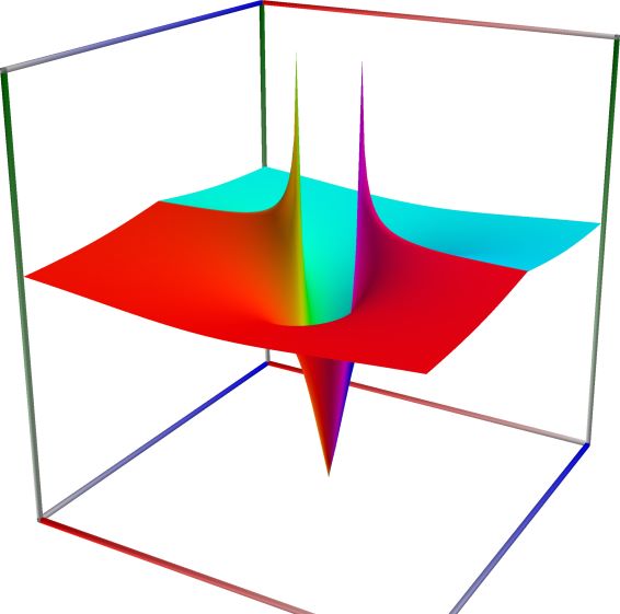

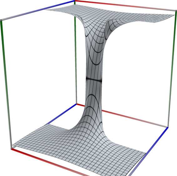
Left figure: real part of the Inverse Tangent function. Camera angles are \(\theta=135^\circ\) and \(\phi = -12^\circ\), camera radius is -2.

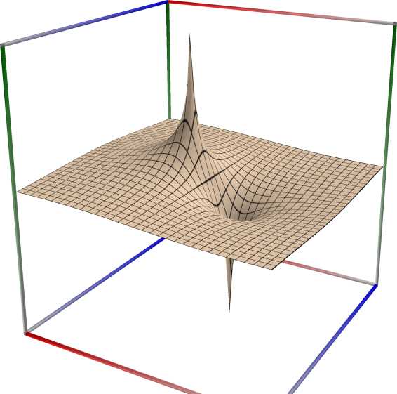
Middle figure: imaginary part of the Inverse Tangent function. Camera angles are \(\theta=135^\circ\) and \(\phi = -12^\circ\), camera radius is -2.

Right figure: absolute value of the Inverse Tangent function, with color-coded phase. Camera angles are \(\theta=135^\circ\) and \(\phi = -12^\circ\), camera radius is -2.

An example in Python

>>> from xlcalcnet import xreal
>>> xreal.Atan(0.5)
xreal('5.2359877559829887307E-1')
>>> xreal.Atan('0.51')
xreal('5.3518479027559984754E-1')

An example in Visual Basic

>>> from xlcalcnet import Gpr
>>> Gpr.Atan(0.5)
Gpr('5.2359877559829887307E-1')
>>> Gpr.Atan('0.51')
Gpr('5.3518479027559984754E-1')

An example with real input:

>>> from xlcalcnet import dec, mpm, ipm
>>> mpm.dps = 40; x = '0.5'
>>> \mathrm{d}x = dec.atan(x); mx = mpm.atan(x); ix = ipm.atan(x)
>>> mpm.show([\mathrm{d}x, mx, ix])
dec:  4.636476090008061162142562314612144020285E-1
mpm:  4.636476090008061162142562314612144020285e-1
ipm:  4.636476090008061162142562314612144020285e-1 (6.19e-40%)

>>> from xlcalcnet import mpm, fpm, gmp, apm
>>> mpm.dps = 40; x = '0.5'
>>> fx = fpm.atan(x); gx = gmp.atan(x); ax = apm.atan(x)
>>> mpm.show([fx, gx, ax])
fpm:  4.63647609000806E-01
gmp:  4.636476090008061162142562314612144020285E-01
apm:  4.636476090008061162142562314612144020285e-1 (6.19e-40%)

The following example with complex input shows that the relative error can be high in double precision:

>>> from xlcalcnet import dec, mpm, ipm
>>> mpm.dps = 20; z = '0.5 + 1.5E-2j'
>>> \mathrm{d}z = dec.atan(z); mz = mpm.atan(z); iz = ipm.atan(z)
>>> mpm.show([\mathrm{d}z, mz, iz], aligned=True)
dec: 4.6371961677714818965E-1             + 1.2000143940891281738E-2j
mpm: 4.6371961677714818965e-1             + 1.2000143940891281738e-2j
ipm: 4.6371961677714818965e-1 (1.37e-19%) + 1.2000143940891281738e-2 (4.853e-18%)j

>>> from xlcalcnet import mpm, fpm, gmp, apm
>>> mpm.dps = 20; z = '0.5 + 1.5E-2j'
>>> fz = fpm.atan(z); gz = gmp.atan(z); az = apm.atan(z)
>>> mpm.show([fz, gz, az], aligned=True)
fpm: 4.63719616777148E-01                  + 1.20001439408913E-02j
gmp: 4.6371961677714818965E-01             + 1.2000143940891281738E-02j
apm: 4.6371961677714818965e-1 (4.567e-20%) + 1.2000143940891281738e-2 (3.309e-19%)j

\(\mathrm{atan}(z)\) is defined so as to be a proper inverse function of \(\tan(\theta)\) for \(-\pi/2 < \theta < \pi/2\). We have \(\tan(\tan^{-1}(x)) = x\) for all \(x\), but \(\tan^{-1}(\tan(x)) = x\) only for \(-\pi/2 < \Re[x] < \pi/2\):

>>> from xlcalcnet import dec, mpr, ivr, ivc
>>> ivr.dps = 25; ivr.pretty = True
>>> mp.dps = 25
>>> for x in [1, 10, -1, 1+3j, -2+3j]:
...     print("%s %s" % (tan(atan(x)), atan(tan(x))))
...
1.0 1.0
10.0 0.5752220392306202846120698
-1.0 -1.0
(1.0 + 3.0j) (1.000000000000000000000001 + 3.0j)
(-2.0 + 3.0j) (1.141592653589793238462644 + 3.0j)

Inverse tangent, 2 arguments, \(\mathrm{atan2}(y, x)\)

ctx.atan2(y, x)

where ctx is math53, mathc53, ctxcpp or ctxflint.

Returns the inverse tangent of \(x\) and \(y\). See also Wikipedia [1379], MathWorld [945], Flint [809], Flint [799], Mpmath [644].

Computes the two-argument arctangent, \(\mathrm{atan2}(y, x)\), giving the signed angle between the positive \(x\)-axis and the point \((x, y)\) in the 2D plane. This function is defined for real \(x\) and \(y\) only.

The two-argument arctangent essentially computes \(\mathrm{atan}(y/x)\), but accounts for the signs of both \(x\) and \(y\) to give the angle for the correct quadrant. The following examples illustrate the difference:

An example in Python

>>> from xlcalcnet import xreal
>>> xreal.Atan2(1,1), xreal.Atan(1/1.)
(0.785398163397448, 0.785398163397448)
>>> xreal.Atan2(1,-1), xreal.Atan(1/-1.)
(2.35619449019234, -0.785398163397448)
>>> xreal.Atan2(-1,1), xreal.Atan(-1/1.)
(-0.785398163397448, -0.785398163397448)
>>> xreal.Atan2(-1,-1), xreal.Atan(-1/-1.)
(-2.35619449019234, 0.785398163397448)

An example in Visual Basic

>>> from xlcalcnet import Gpr
>>> Gpr.Atan2(1,1), Gpr.Atan(1/1.)
(0.785398163397448, 0.785398163397448)
>>> Gpr.Atan2(1,-1), Gpr.Atan(1/-1.)
(2.35619449019234, -0.785398163397448)
>>> Gpr.Atan2(-1,1), Gpr.Atan(-1/1.)
(-0.785398163397448, -0.785398163397448)
>>> Gpr.Atan2(-1,-1), Gpr.Atan(-1/-1.)
(-2.35619449019234, 0.785398163397448)

The angle convention is the same as that used for the complex argument.

Inverse cotangent, \(\mathrm{acot}(x)\)

ctx.acot(x)

Returns the inverse cotangent of \(x\), \(\mathrm{acot}(x)\). See also Wikipedia [1366], MathWorld [942], NIST [512], Ehrhardt [309] (4.2.5).

\(\quad\) \(\quad\)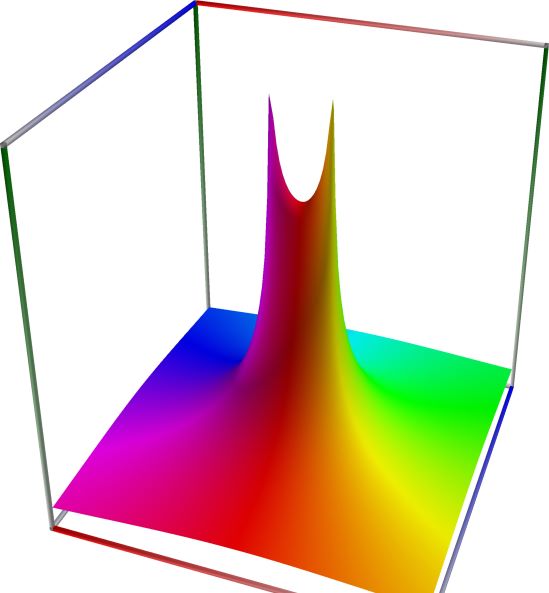

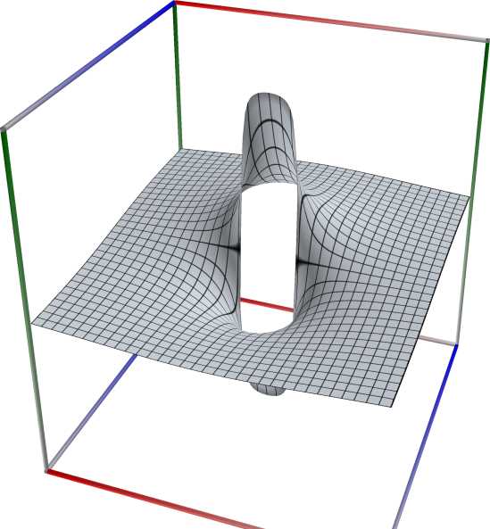
Left figure: real part of the Inverse Cotangent function. Camera angles are \(\theta=135^\circ\) and \(\phi = -12^\circ\), camera radius is -2.

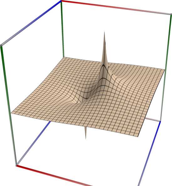
Middle figure: imaginary part of the Inverse Cotangent function. Camera angles are \(\theta=135^\circ\) and \(\phi = -12^\circ\), camera radius is -2.

Right figure: absolute value of the Inverse Cotangent function, with color-coded phase. Camera angles are \(\theta=135^\circ\) and \(\phi = -12^\circ\), camera radius is -2.

The inverse cotangent can be expressed in terms of the inverse tangent as \(\displaystyle \mathrm{acot}(x) = \mathrm{atan}\left(\frac{1}{x} \right)\). This is a real-valued function for all real \(x\), with range \((0, \pi)\).

The inverse cotangent can be expressed in terms of related functions (with the principal-branch log and square root):

\[\mathrm{acot}(z) = \frac{i}{2} \left[ \log \left(1 - \frac{i}{z} \right) - \log \left(1 + \frac{i}{z} \right) \right]= \mathrm{atan}\left(\frac{1}{z}\right)\]

An example in Python

>>> from xlcalcnet import xreal
>>> xreal.Acot(0.5)
xreal('5.2359877559829887307E-1')
>>> xreal.Acot('0.51')
xreal('5.3518479027559984754E-1')

An example in Visual Basic

>>> from xlcalcnet import Gpr
>>> Gpr.Acot(0.5)
Gpr('5.2359877559829887307E-1')
>>> Gpr.Acot('0.51')
Gpr('5.3518479027559984754E-1')

An example with real input:

>>> from xlcalcnet import dec, mpm, ipm
>>> mpm.dps = 40; x = '2.0'
>>> \mathrm{d}x = dec.asec(x); mx = mpm.asec(x); ix = ipm.asec(x)
>>> mpm.show([\mathrm{d}x, mx, ix])
dec:  1.047197551196597746154214461093167628066E+0
mpm:  1.047197551196597746154214461093167628066e+0
ipm:  1.047197551196597746154214461093167628066e+0 (1.096e-39%)

>>> from xlcalcnet import mpm, fpm, gmp, apm
>>> mpm.dps = 40; x = '2.0'
>>> fx = fpm.asec(x); gx = gmp.asec(x); ax = apm.asec(x)
>>> mpm.show([fx, gx, ax])
fpm:  1.04719755119660E+00
gmp:  1.047197551196597746154214461093167628066E+00
apm:  1.047197551196597746154214461093167628066e+0 (1.096e-39%)

The following example with complex input shows that the relative error can be high in double precision:

>>> from xlcalcnet import dec, mpm, ipm
>>> mpm.dps = 20; z = '2.0 + 1.5E-2j'
>>> \mathrm{d}z = dec.asec(z); mz = mpm.asec(z); iz = ipm.asec(z)
>>> mpm.show([\mathrm{d}z, mz, iz], aligned=True)
dec: 1.0472354363409255922E+0              + 4.3297752322606827325E-3j
mpm: 1.0472354363409255922e+0              + 4.3297752322606827325e-3j
ipm: 1.0472354363409255922e+0 (2.426e-19%) + 4.3297752322606827323e-3 (3.508e-17%)j

>>> from xlcalcnet import mpm, fpm, gmp, apm
>>> mpm.dps = 20; z = '2.0 + 1.5E-2j'
>>> fz = fpm.asec(z); gz = gmp.asec(z); az = apm.asec(z)
>>> mpm.show([fz, gz, az], aligned=True)
fpm: 1.04723543634093E+00                  + 4.32977523226068E-03j
gmp: 1.0472354363409255922E+00             + 4.3297752322606827325E-03j
apm: 1.0472354363409255922e+0 (8.088e-20%) + 4.3297752322606827324e-3 (1.146e-18%)j

Inverse cosecant, \(\mathrm{acsc}(x)\)

ctx.acsc(x)

where ctx is math53, mathc53, ctxcpp or ctxflint.

Returns the inverse cosecant of \(x\), \(\mathrm{acsc}(x)\). See also Wikipedia [1366], MathWorld [940], NIST [512], Ehrhardt [309] (4.2.9), Mpmath [594].

The inverse cosecant can be expressed in terms of the inverse sine as \(\displaystyle \mathrm{acsc}(x) = \mathrm{asin}\left(\frac{1}{x} \right)\). The domain is \(\displaystyle \mathbb {R} \setminus (-1,1)\), i.e. \(|x|>0\).

The inverse cosecant can be expressed in terms of related functions (with the principal-branch log and square root):

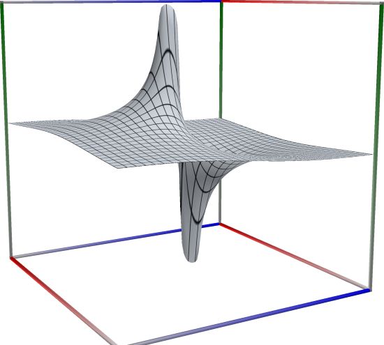
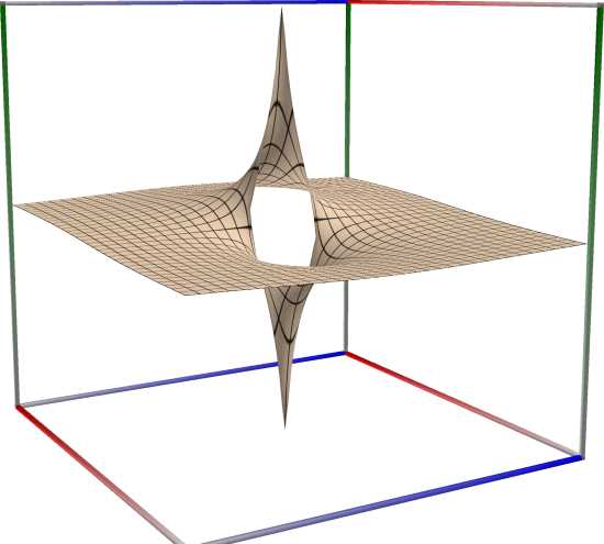
\[\mathrm{acsc}(z) = -i \log \left( \sqrt{1-\frac{1}{z^2}} + \frac{i}{z} \right) = \mathrm{asin}\left(\frac{1}{z}\right)\]

\(\quad\) \(\quad\)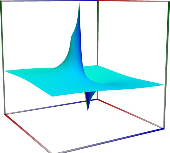

Left figure: real part of the Inverse Cosecant function. Camera angles are \(\theta=135^\circ\) and \(\phi = -12^\circ\), camera radius is -2.

Middle figure: imaginary part of the Inverse Cosecant function. Camera angles are \(\theta=135^\circ\) and \(\phi = -12^\circ\), camera radius is -2.

Right figure: absolute value of the Inverse Cosecant function, with color-coded phase. Camera angles are \(\theta=135^\circ\) and \(\phi = -12^\circ\), camera radius is -2.

An example in Python

>>> from xlcalcnet import xreal
>>> xreal.Acsc(0.5)
xreal('5.2359877559829887307E-1')
>>> xreal.Acsc('0.51')
xreal('5.3518479027559984754E-1')

An example in Visual Basic

>>> from xlcalcnet import Gpr
>>> Gpr.Acsc(0.5)
Gpr('5.2359877559829887307E-1')
>>> Gpr.Acsc('0.51')
Gpr('5.3518479027559984754E-1')

An example with real input:

>>> from xlcalcnet import dec, mpm, ipm
>>> mpm.dps = 40; x = '2.0'
>>> \mathrm{d}x = dec.acsc(x); mx = mpm.acsc(x); ix = ipm.acsc(x)
>>> mpm.show([\mathrm{d}x, mx, ix])
dec:  5.235987755982988730771072305465838140329E-1
mpm:  5.235987755982988730771072305465838140329e-1
ipm:  5.235987755982988730771072305465838140329e-1 (2.192e-39%)

>>> from xlcalcnet import mpm, fpm, gmp, apm
>>> mpm.dps = 40; x = '2.0'
>>> fx = fpm.acsc(x); gx = gmp.acsc(x); ax = apm.acsc(x)
>>> mpm.show([fx, gx, ax])
fpm:  5.23598775598299E-01
gmp:  5.235987755982988730771072305465838140329E-01
apm:  5.235987755982988730771072305465838140329e-1 (1.096e-39%)

The following example with complex input shows that the relative error can be high in double precision:

>>> from xlcalcnet import dec, mpm, ipm
>>> mpm.dps = 20; z = '2.0 + 1.5E-2j'
>>> \mathrm{d}z = dec.acsc(z); mz = mpm.acsc(z); iz = ipm.acsc(z)
>>> mpm.show([\mathrm{d}z, mz, iz], aligned=True)
dec: 5.2356089045397102702E-1              - 4.3297752322606827325E-3j
mpm: 5.2356089045397102702e-1              - 4.3297752322606827325e-3j
ipm: 5.2356089045397102702e-1 (4.045e-19%) - 4.3297752322606827323e-3 (-3.508e-17%)j

>>> from xlcalcnet import mpm, fpm, gmp, apm
>>> mpm.dps = 20; z = '2.0 + 1.5E-2j'
>>> fz = fpm.acsc(z); gz = gmp.acsc(z); az = apm.acsc(z)
>>> mpm.show([fz, gz, az], aligned=True)
fpm: 5.23560890453971E-01                  - 4.32977523226068E-03j
gmp: 5.2356089045397102702E-01             - 4.3297752322606827325E-03j
apm: 5.2356089045397102702e-1 (8.089e-20%) - 4.3297752322606827324e-3 (-1.146e-18%)j

Inverse secant, \(\mathrm{asec}(x)\)

ctx.asec(x)

where ctx is math53, mathc53, ctxcpp or ctxflint.

Returns the inverse secant of \(x\), \(\mathrm{asec}(x)\). See also Wikipedia [1366], MathWorld [943], NIST [512], Ehrhardt [309] (4.2.11), Mpmath [603].

The inverse secant can be expressed in terms of the inverse cosine as \(\displaystyle \mathrm{asec}(x) = \mathrm{acos}\left(\frac{1}{x} \right)\). The domain is \(\displaystyle \mathbb {R} \setminus (-1,1)\), i.e. \(|x|>0\).

The inverse secant can be expressed in terms of related functions (with the principal-branch log and square root):

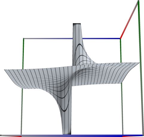
\[\mathrm{asec}(z) = -i \log \left( \sqrt{\frac{1}{z^2}-1} + \frac{1}{z} \right) = \mathrm{acos}\left(\frac{1}{z}\right)\]

\(\quad\) \(\quad\)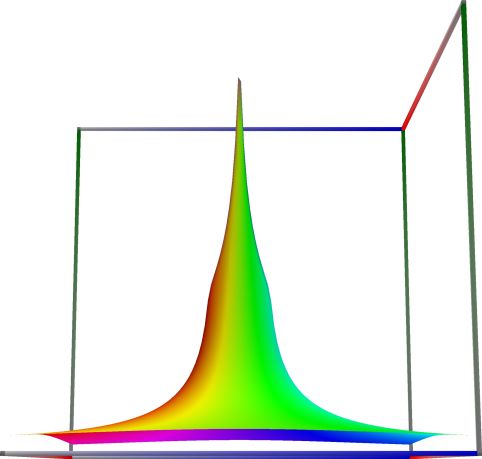

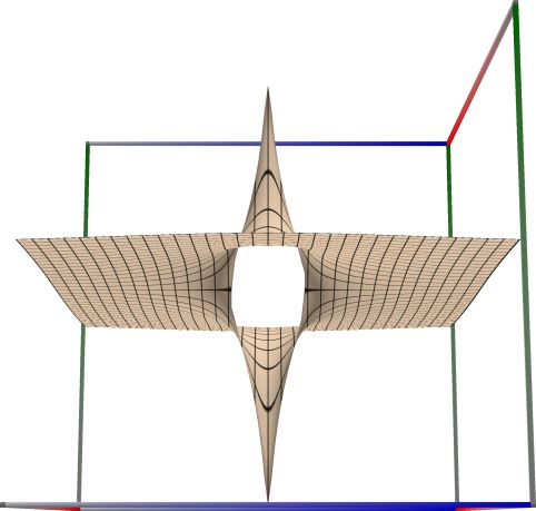
Left figure: real part of the Inverse Secant function. Camera angles are \(\theta=135^\circ\) and \(\phi = -12^\circ\), camera radius is -2.

Middle figure: imaginary part of the Inverse Secant function. Camera angles are \(\theta=135^\circ\) and \(\phi = -12^\circ\), camera radius is -2.

Right figure: absolute value of the Inverse Secant function, with color-coded phase. Camera angles are \(\theta=135^\circ\) and \(\phi = -12^\circ\), camera radius is -2.

An example in Python

>>> from xlcalcnet import xreal
>>> xreal.Asec(0.5)
xreal('5.2359877559829887307E-1')
>>> xreal.Asec('0.51')
xreal('5.3518479027559984754E-1')

An example in Visual Basic

>>> from xlcalcnet import Gpr
>>> Gpr.Asec(0.5)
Gpr('5.2359877559829887307E-1')
>>> Gpr.Asec('0.51')
Gpr('5.3518479027559984754E-1')

An example with real input:

>>> from xlcalcnet import dec, mpm, ipm
>>> mpm.dps = 40; x = '2.0'
>>> \mathrm{d}x = dec.asec(x); mx = mpm.asec(x); ix = ipm.asec(x)
>>> mpm.show([\mathrm{d}x, mx, ix])
dec:  1.047197551196597746154214461093167628066E+0
mpm:  1.047197551196597746154214461093167628066e+0
ipm:  1.047197551196597746154214461093167628066e+0 (1.096e-39%)

>>> from xlcalcnet import mpm, fpm, gmp, apm
>>> mpm.dps = 40; x = '2.0'
>>> fx = fpm.asec(x); gx = gmp.asec(x); ax = apm.asec(x)
>>> mpm.show([fx, gx, ax])
fpm:  1.04719755119660E+00
gmp:  1.047197551196597746154214461093167628066E+00
apm:  1.047197551196597746154214461093167628066e+0 (1.096e-39%)

The following example with complex input shows that the relative error can be high in double precision:

>>> from xlcalcnet import dec, mpm, ipm
>>> mpm.dps = 20; z = '2.0 + 1.5E-2j'
>>> \mathrm{d}z = dec.asec(z); mz = mpm.asec(z); iz = ipm.asec(z)
>>> mpm.show([\mathrm{d}z, mz, iz], aligned=True)
dec: 1.0472354363409255922E+0              + 4.3297752322606827325E-3j
mpm: 1.0472354363409255922e+0              + 4.3297752322606827325e-3j
ipm: 1.0472354363409255922e+0 (2.426e-19%) + 4.3297752322606827323e-3 (3.508e-17%)j

>>> from xlcalcnet import mpm, fpm, gmp, apm
>>> mpm.dps = 20; z = '2.0 + 1.5E-2j'
>>> fz = fpm.asec(z); gz = gmp.asec(z); az = apm.asec(z)
>>> mpm.show([fz, gz, az], aligned=True)
fpm: 1.04723543634093E+00                  + 4.32977523226068E-03j
gmp: 1.0472354363409255922E+00             + 4.3297752322606827325E-03j
apm: 1.0472354363409255922e+0 (8.088e-20%) + 4.3297752322606827324e-3 (1.146e-18%)j